Financial Centres’ Polyarchy and
Competitiveness
Does Political Participation Change a Financial Centre’s
Competitiveness?
Bryane Michael
University of Oxford
Bertrand Candelon
University Maastricht and Université Catholique de Louvain
Abstract
What role does polyarchy (and thus increased democracy) play in aiding the development of an international financial centre? We find support for decades of theorising that some jurisdictions use autocracy (less polyarchy) to help grow out their financial centres. We look at the growth of these financial centres as the extent to which they attract more funds from abroad (cross-border bank liabilities). Polyarchy decreases as other international financial centres’ centrality in the global financial centre network expands. Polyarchy increases in most jurisdictions over time because some financial centres rely on increasingly polyartic governance as a way to foster financial innovation through increased participation by non-previously powerful sectors. Namely, the growth of an international financial centre’s centrality in global financial networks relies on tapping down on polyarchy. Yet, such polyarchy – when used by some very central jurisdictions to remain central – “spreads.” We model such a relationship between polyarchy and centrality in the global financial network, describing even the most complex quantitative analysis in a way a non-specialist can understand. These results could impact decisions ranging from Brexit to Hong Kong’s autonomy in its post-2047 period.
Keywords: international financial centres, endogenous global city network centrality, dynamic polyarchy, finance juntas, financial competitiveness, Bayesian network analysis.
JEL Codes: D72, F55, F33, P48
We acknowledge the Hong Kong University Grant Council’s
Theme-Based Research Scheme for partially funding this research under the
research programme Enhancing Hong Kong's Future as a Leading International
Financial Centre. We also acknowledge support from the Europlace Institute
of Finance and Insti7 programme Risk Management, Investment Strategies and
Financial Stability. All ideas, as well as any omissions and mistakes,
remain our own. We do not claim to represent the views of any institutions we
affiliate with, and nothing in this paper represents investment advice. Co-authors
have worked on separate sections of the paper (as a multi-disciplinary
project), thus each co-author may not necessarily agree with all the material
in the paper.
Contents
The Blundering Literature on Political Institutions and
International Financial Centres
From regressions on democracy to political cycles
Looking for democratic/polyartic cycles as politicians
promise more foreign investment
The Stylized Facts: The Link between Democratic Inclusion
and Financial Centre Competitiveness
Democracy in Y/Zen’s top international financial centres
Polyarchy and international financial centres
Modelling and Operationalizing Endogenous Change in IFC
Politics and Competitiveness
Changes Within and Between Countries
The Data and Empirical Methods We Used
Jurisdictions, raw polyarchy and network centralities
Getting polyarchy and network centralities ready for
analysis
Does Polyarchy React to a Financial Centre’s Centrality?
How Reliable Are These Results?
Appendix I: A Model of Domestic Political Change and a
Model of Network Change
The micro-foundations of financial assets versus
polyarchy
Supply and demand for polyarchy, innovation and
investment assets
Modelling the interference from covariates
Appendix II: Details of Econometric Procedures and
Results
Fitting
the macro and other factors to the data
Variables used to create network data
Matrix Statistics for Banking Liability Data
Polyarchy and Importance to the Financial Network
Financial Centres’ Polyarchy and
Competitiveness
Does Political Participation Change a Financial Centre’s
Competitiveness?
Bryane Michael, University of Oxford
Bertrand Candelon, University Maastricht and Université Catholique de Louvain
Introduction
Democratic institutions seem antithetical to building world-class international financial centres. Most famously, Shaxson – in his survey of tax havens – notes the extent to which secret cabals in The City (in London), Delaware, Jersey and other places dominated financial services lawmaking.[1] Regulatory capture has resulted in financial regulations which have made several international financial centres far more competitive – if far less robust to crises -- and less consumer-friendly.[2] The need to grow local financial centres into internationally competitive international financial centres has subsumed local politics in many places – resulting in the tacit or explicit restriction of certain political ideas and polities.[3] Even in places not usually considered as financial centres until recently, the design of regulatory institutions has encouraged such capture.[4] Politics -- dominated by elites, specialists and/or special interest groups -- has determined the extent and type of financial regulations in international financial centres.[5] Indeed, some have argued that policies aimed at making an international financial centre more competitive have helped some of these groups stay in power and forestall political rivalry.[6] To what extent does international financial centres’ competitiveness incentivize/enable such restrictions on political pluralism? To what extent does the reverse happen – as restrictions on political participation boost the competitiveness of the financial centres which legitimizes certain politically powerful groups?
Our paper shows that political participation in adjusts to a financial centre’s competitiveness, and that competition between international financial centres affects the extent of such political participation/pluralism in these financial centres. For example, Hong Kong lawmakers and politicians may keep a close eye on how many assets London, New York and Singapore-based asset managers attract from abroad – shutting down groups vying for other interests (like income redistribution) when Hong Kong’s own competitiveness falls. Decisions about political pluralism and financial centre performance seem inexorably linked in leading financial centres, not only within these centres but also between them.[7] Yet, greater political participation/inclusiveness does not always/only reduce the performance/competitiveness of an international financial centre. The inclusion of different ideas and interests does not only drag down performance. As costs and benefits in the international network of financial centres changes, so must individual centres adapt – renewing the services and systems they use to compete globally. Increasingly democratic political institutions help foment these new ideas.[8] Political competition and plurality helps generate new ideas for improving the intermediation of capital, as well as support for the financial centre. As these financial centres attract more assets and thus profits, they have more gains to share among different constituencies who demand rewards for their previous patient silence. When a financial centre reaches a certain size, more polyartic institutions allow the winners to compensate other sectors of society, as well as draw them in into a process for seeking their ideas and political support for new and better ways of competing internationally.[9] Political plurality and international centre competitiveness are thus locked in a dynamic dance across time. Any proposal to reform financial institutions thus needs to match the phase of that dance in order to achieve its desired effects. Policymakers in places like the UK and Hong Kong need not ask whether they should keep or give up greater autonomy over their financial regulation. The main question concerns whether they need to make this adjust right now.
We draw together the data into a conjecture about the way that international financial centres’ competitiveness and polyarchy interact across these centres. We measure such competitiveness as the cross-border assets drawn in by international financial centres’ banks. We use an off-the-shelf measure of polyarchy, as the extent to which more groups affect (or are allowed to affect) policy.[10] We conjecture that these international financial centres need to restrict such polyarchy to pass the narrow financial regulations needed to grow the national financial centre(s).[11] As other financial centres do the same thing – lawmakers, politicians and regulators need new ideas for financial sector regulations that will give them the edge. Such ideas come from the fracas of political competition, from new polities and the need to strike compromises.[12] Yet, polyarchy reduces again as governments of the day need to reduce resistance toward implementing these new ideas.[13]
We structure the paper as follows. First, we review the scant theorising about international financial centre competitiveness (size, growth, market niches and so forth) and their political plurality. Hundreds of political theorists, historians and geographers have written about the way that political interest groups use financial policies to obtain and keep political power. Yet, we could find none looking at the use of these policies at the global level (between financial centres themselves). Second, we look at trends in the raw data before going into our in-depth analysis. These trends set the stage for our main analysis, and should provide the reader with the intuitions and insights needed to assess our later analysis. The third section presents our model – showing how we see the trade-off between innovation and ‘focus’ (for lack of a better word). As usual in economics, jurisdictions have an optimal amount of polyarchy at any given time – polyarchy which helps attract the larger amount of cross-border bank liabilities given the polyarchy and central of other financial centres in global financial centre networks. The fourth section explains our empirical methods, using language simple enough for a non-social scientist to understand.[14] The final section concludes. The appendices offer more quantitative background and support for our analysis.
We should caution the reader about some assumptions we make before beginning our argument. First, we must assume that political polyarchy at the ballet box in some way reflects polyarchy of those groups, cabals, juntas, bureaucrats and bankers who make financial policy.[15] We understand the limitations of assuming that Swedish financial interests must vary more than Chinese ones – even though China has far more stakeholder groups interested in the outcomes of financial policy than Sweden has.[16] Even though Saudi Arabia (for example) does not hold open elections often, elite rivalries do shape financial policy, as patrons on behalf of their clients and supporters – and they influence financial policies polyartically at the Cabinet of Ministers and ministerial levels.[17] Where possible, we provide references to previous research showing the usefulness and likely validity of such an assumption on the macro-level. Similarly, albeit more credibly, we hypothesize that when polyarchy decreases, financial regulation reflects the interests of the groups in power. In other words, we do not distinguish between differences in power between groups exercising polyartic power. Nevertheless, we do not assume that the members of a particular polyarchy reflect mostly financial institutions’ interests (indeed we test this proposition in our paper). We may also slip by associating more polyarchy with more democracy – a fact true by definition except when a jurisdiction changes from a position of greater to less democracy (thus becoming more autocratic).[18] We may also slip by talking about V-Dem’s polyarchy measure as a more reliable measure of the polyarchy want to understand than it is.[19]
Our other assumption major assumption deals with the way more polyarchy translates into more financial innovation (or at least competitiveness). We empirically test the extent to which polyarchy correlates with a financial centre’s centrality – particularly for very large and central jurisdictions with rising polyarchy. We theorise that polyarchy’s benefit comes from financial innovation and good ideas from a larger range of society’s stakeholders – rather than from something else. Based on our literature review, this looks like a reasonable assumption.[20] However, we usual refer to this chain of causation, while ignoring other possibilities.[21] To keep our paper at a reasonable length, we do not try to figure out the exact reason why polyarchy might rise after a time of repression, when the financial centre becomes larger.[22]
Another assumption concerns our definition of financial centre competitiveness. We equate cross-border banking liabilities with a jurisdiction’s competitiveness. Yet, we use Y/Zen’s list of top international financial centres to choose the jurisdictions to study – a list which most decidedly rejects such a narrow definition.[23] Indeed, as we show later in our paper, cross-border bank liabilities flows differ from the flows of assets, equity, short-term and long-term debt. With some jurisdictions specialising in securitisation, mutual funds, and foreign exchange, our approach captures a microscopic part of this overall competitiveness.[24] We feel justified though in talking about broader competitiveness, as our methodology easily extends to these markets. Many financial centres excel in many financial services at the same time because of their “product complementarities, the nature of local epistemic communities, and regulation.”[25]
Finally, we often must talk about international financial centres (like Frankfort or Paris) using data for their nation-state (Germany and France respectively). For jurisdictions with multiple financial centres -- like the US, China, and Germany – using national polyarchy hardly represents a fair portrayal of polyarchy on Wall Street (New York) versus Sand Hill Road (San Francisco). Doha, Seoul or Tokyo might (or might not) account for most of these jurisdictions’ banking centrality. Lack of data at the city-level forces us to elide entire jurisdictions with the city that appears on Z/Yen’s index of top international financial centres. We try to refer to the country as a whole, rather than individual financial centres – leaving it up to the reader and future researchers as to the extent to which the jurisdiction’s whole represents its parts as metropolitan financial centres.[26]
The
Blundering Literature on Political Institutions and International Financial
Centres
From regressions on democracy to political cycles
None of the studies of international financial centres look directly, quantitatively or econometrically at the way local political institutions respond to the competitiveness of their international financial centres. Did Singapore’s and Lee Kwan Yew’s People’s Action Party’s resistance to outside and variegated political participation help the nation-state’s elites build a world-class financial centre? How much did the politics of Wall Street’s elites drive Ronald Reagan’s liberalisation programme (and his chocking off to participatory policymaking institutions like labour unions’ input into policy)? How much did the need to compete with Tokyo or London also shape the former US President’s decisions? Despite extensive work on measuring and assessing international financial centres, previous studies tend to ignore three aspects of international financial centre competitiveness politics. First, to the extent they empirically/econometrically look at the link between politics and international financial centre competitiveness, they do so through the lens of “democracy.” Second, they ignore the dynamics of political change – and the way that political change drives international financial centre competitiveness. Third, they ignore local politics responds to and affects local politics abroad as these politicians look at the competitiveness of their jurisdictions’ financial institutions.
The first blunder of the literature
consists of a narrow focus on regressions looking at the relationship between democracy
and financial development.[27]
For example, studies like Doces looked at the extent to which differing levels
of a survey indicator designed to proxy the extent/level of ‘democracy’
correlated with levels of foreign direct investment.[28]
Girma and Shortland might find that the degree of democracy (or elite capture
of political decisions) affects financial sector development, as measured by
indicators such as private sector credit-to-GDP ratios, stock market
capitalisation-to-GDP ratios and stock market value traded-to-GDP ratios.[29]
Democracy and “good” political institutions – holding other variables fixed –
aid in financial sector development and thus the likely emergence of
international financial centres.[30]
Yet, the consensus – if one can call it a consensus – finds that democracy
helps promote the development of large financial sectors using measures like
these, only for countries with robust legal and governance institutions in
place.[31]
Democratic development and financial sector/market development have gone together
since the industrial revolution, and will likely continue to do so.[32]
Of course dissenters and hedgers will always remain, given the messy nature of
the world and the data.[33]
The nature of these measures also pose problems, as indicators measuring the extent
to which a country has an autocratic versus democratic governance institutions,
as well as measures which try to measure the durability of those institutions,
remain highly problematic.[34]
Yet, these studies fail in a more fundamental way. They fail to look at
dynamics – how the extent of democracy and self-determination change over time
in response to changing investment needs.[35]
The second blunder of the literature consists of ignoring the dynamics of changing financial sector competitiveness and political participation. Many works – particularly by geographers – talk about cycles of political participation and financial sector competitiveness over time, from an economic, political and sociological perspective. Any study of a financial centre, like Singapore, would show the constant competition with other financial centres, the need for politicians to restrict or expand democratic participation as needed, and the way that such participation affects an international financial centre’s competitiveness.[36] In the US context, scholars and pundits alike see a dichotomy between “democratic participation” in finance and a more centralised one, focused around finance-sector interest groups.[37] Many of these focus on events which depend as much as historical accident as any deliberate policies arising after, or in reaction to, these accidents. Subsequent policy may encourage the development of a financial centre.[38] Yet, few provide a working, testable model of political and financial sector change in international financial centres. Some exceptions do exist.[39] Yet, many describe such accidents as “path dependencies” (meaning we don not know really if their causes can be replicated).[40] Yet, a large literature even exists admonishing academics with quantitative research skills to pay attention to the inter-relationship between politics and finance in the development and growth of these international financial centres...leading to our third blunder.[41]
The third blunder committed by the literature in our subject consists of most discussions tending to depoliticise both the national and international aspects of international financial centres.[42] At their most extreme, models of financial centres see different policies ‘diffusing’ – with financial authorities copying policies from other jurisdictions like the spreading of a fad or hit song.[43] Such diffusion has no room for politics, either within or between jurisdictions. For authors like Hampton and Christensen, the politics of these international financial centres extends only so far as such lobbying (usually targeted at tax havens) help or hurt other – particularly larger – countries like the US.[44] They describe how the IMF, the OECD and even countries like the US call for financial and other reforms in the international financial centres.[45] They draft the rules that countries can follow – or not.[46] Many even argue that international elites use and abuse these centres and their places – in effect usurping their politics.[47] Others argue that local elites manipulate the political process – without ever describing who or how -- to create an international financial centre serving their own interests.[48] These elites’ better understanding of the complexities of finance (better than even national regulators) supposedly facilitate their ability to manipulate the political process and the government itself.[49] If international financial centres do compete, authors like Hall would have us believe that they do so through apolitical government policies.[50] Wang and authors of his ilk present the results of such political machinations and movements as faits accomplis (the inevitable result and cause of “political will”).[51]
Worse still, they ignore the strong political as well as economic harms many of these reforms would cause if local politicians did more than pay these reforms lip service. For these authors, the most that can happen is that, “the cumulative pressures for reform will significantly re-configure the offshore finance industry. Offshore finance may return onshore to the large, functional financial centers such as London or New York.”[52] Such a reshoring would kill many political careers in these centres. Many international financial centres seem to exist to serve as offshore international financial centres – making their success a prime political objective.[53] Authors that claim that such competition simply represents “jurists' and policymakers' attempts to resolve an inherent contradiction between insulated state law and the rapidly integrating world market” have been as misled as these politicians’ constituents into believing financial law represents a non-political, non-competitive ‘policy area.’[54]
To understand the dynamics of political change, given economic/commercial change in an international financial centre, we must turn toward the historical literature. Recent case study and historical treatments of financial centre development have particularly shown the waving and waning nature of democracy and financial sector development. Financial, and thus economic, performance represents a strong electoral issue in many countries – just as electoral results represent strong drivers of international portfolio and direct investment.[55] Politicians and any/all interested parties keep an eye on the rhetoric and policies foreign investors want.[56] Sometimes, such competition between international financial centres may imperil the viability of the policies these jurisdictions have put in place to compete internationally in the first place.[57] While many emerging markets “simply do not exist for global financial market investors,” some financial centres absolutely do.[58] Many of these political and foreign investment decisions follow cycles. Most scholars have assumed that the uncertainty in these cycles drive investment.[59] But what if the decisions taken in these cycles reflect the nature of the cycle itself? Namely, what if disposition toward particular political practices and institutions (particularly democratic ones) cause changes in investment – which in turn – causes changes in political preferences?[60]
Looking for democratic/polyartic cycles as politicians
promise more foreign investment
The British Virgin Islands provides one concrete example, showing how the politics of an international financial centre depend on that centre’s ranking vis-a-vis other centres (and the difficulty of empirically detecting such dependency). Like many of the top international financial centres, the British Virgin Islands (BVI) has inherited a historical focus on international finance due to its position along trading routes and its specialisation in a larger political/economic entity (the British Empire).[61] In the classical telling of BVI’s inherited position as an international financial centre, the jurisdiction – like the other crown dependencies – had served as an extension of the City of London.[62] Like in the Cayman Islands, groups vied for power by giving foreigners tax and other benefits in exchange for bringing their money to the island.[63] Yet, as shown in Figure 1, these policies had less impact then similar policies in the Cayman Islands, Jersey, Bermuda and the other jurisdictions shown in the figure. The BVI’s GDP and employment share of finance hovered at around 10% of GDP at the start of this decade. Doubtlessly, the BVI’s falling behind other financial centres at the time of the global financial crisis, and long before then, influenced the Island’s politicians far more than this sector’s meagre size suggests. The financial sector almost certainly influences local politicians more than its small size to GDP suggests. [64]
In fact, national politicians used the jurisdiction’s nascent financial development as both political end and means. Orlando Smith, at the start of the millennium, intensified the trend already underway of cooperating with business interests, cleaning up corruption, and most prominently working to grow the Island’s offshore financial industry.[65] His National Democratic Party won the 2003 general election (having formed to run in the previous election of 1999). While he and his party did not win the next elections in 2007, they proved instrumental in ratify a new constitution by the time of the 2007 election. True to BVI politics, neither the National Democratic Party, nor the incumbent Virgin Islands Party focused on the development of offshore finance on ideological grounds. Instead, as noted by several commentators, politics has focused on personal connections, charisma and most importantly -- patronage. As such, the new constitutional project did not appear out of some deep-seated philosophical struggle. The effects of the new constitution – and subsequent laws passed under it – included putting foreign investors and financiers at ease by offering protections against arbitrary seizure/nationalisation of their property rights and investments as well as unwelcome interference from the UK.[66] As in other places, foreign politicians fed this internal political dynamic, as these financial centres served their personal and national pecuniary interests.[67]
Yet, even for a small jurisdiction like the BVI, finding any direct link between politics and foreign investment proves difficult. Figure 2 shows the electoral share of the National Democratic Party (NDP), its main rival the Virgin Islands Party (VIP) and portfolio investment from the US and UK.[68] Despite over-whelming support for the VIP around 2007, US investment shrank (with UK investment radically rising). At the beginning of the 2000s and in recent years, the NDP has won elections, coinciding with slower growth (or even shrinkage) of such portfolio investment. The 2004 BVI Business Companies Act came on the books on the NDP’s watch (though fully implemented by the time the VIP won power).[69] Offshore finance – and offshore company registrations – provided about 55% of total government revenues (amounting to a bit over US$187 million) around that time.[70] No matter which political party held power, the BVI represented a “captured state.”[71] The particular party in power mattered far less for the passage of competitive legislation like the 2003 Virgin Islands Special Trusts Act or non-enforcement of due diligence rules than the extent of political competition.[72]
The lack of political competition and thus effective democracy in any international financial centres, has given financial interests very large influence over financial policies. The BVIs do not quite epitomize the state capture attributed to Jersey.[73] Centres like Jersey allow us to witness the way such capture transcends borders – showing the dependence of financial centres’ politics and policies on each other. International services firms’ (like Price Waterhouse and Ernst & Young) push to expand rules enabling financial centres like Jersey show the extent of global pressure on financial centres.[74] Jersey, in this case, clearly reacted to developments in other jurisdictions. Just like Jersey, other financial centres’ politicians point to the BVIs as model, rival and legitmiser.[75]
The lack of effective multi-party democratic decision-making in some places leaves them open to influence from/through these other channels. Politics represents a contest over financial policy – and finance itself.[76] Less vigorous political competition may allow the state capture which promotes the financial sector competitiveness of places like the BVI and Jersey. Yet, preferences for such political competition do not exist in a vacuum.
Economic forces affect the extent of political competition. Figure 3 shows support for a democratic political system in the jurisdictions housing most of the financial centres we study.[77] US and Japanese voters/citizens view democracy less favourably after the global financial crisis. Relatively untouched jurisdictions like Sweden and Hong Kong have had greater support for democracy over time. A simple bar chart does not prove that democratic or polyartic governance responds to changes in economic factors or a jurisdiction’s financial sector’s competitiveness. Yet, preferences for – and responses to – democratic and polyartic governance do change over time in response to economic change and visa versa.[78] What do the data tell us?

The
Stylized Facts: The Link between Democratic Inclusion and Financial Centre
Competitiveness
Democracy in Y/Zen’s top international financial centres
Superficial data show that international financial centres need just the right amount of democracy at just the right time to thrive. Figure 4 shows the most simplistic analysis available – a popular survey-based measure of international financial centres’ competitiveness versus a measure of the extent of democracy in the international financial centres’ jurisdiction.[79] ‘Authoritarian’ (their words, not ours) leaders like China and the United Arab Emirates sit at one end of the spectrum.[80] Legitimacy-by-performance might drive any attempt to create an international financial centre (as authoritarian governments seek to bolster their rule by creating sectors that push up national income).[81] Gibraltar and the Bahamas, as ‘contender democracies,’ sit at the other end of the spectrum.[82] According to this static picture, taken in 2016, the largest number of highly competitive ‘leader’ jurisdictions came from ‘flawed’ democracies. ‘Hybrid democracies’ had the hardest time breaking into the ranks of the international financial centre leaders. Such difficulty probably reflects both their fragility and the resources going into ‘stage managing’ the political/electoral system.[83] Most importantly, different political regimes statistically significantly correspond with a particular type of financial centre.[84] In other words, leader financial centres grow up around democratic governments statistically significantly more often than they do in authoritarian governments.

More specific data seems to show that democracy hurts financial centre competitiveness. Figure 5 moves from comparing categories to comparing numerical measurements of the extent of democracy and the competitiveness of international financial centres. The same rough pattern emerges. From such a static picture, we see that relatively uncompetitive financial centres have all kinds of governments – from the very democratic to the not-so-much. Yet, the most competitive financial centres in the mid-2010s had more democratic governments (as represented by the countries at the top of the pyramid of dots on the right hand side of the figure). Such figures immediately dispel any monolithic theory positing that globalisation somehow leads to the degeneration of democracy.[85] Nothing in these data point to a supposed contradiction between financial globalisation and democracy.[86]
What happens to the odds of an international financial centre becoming more competitive as it becomes more democratic? Figure 6 shows the “risk” of an international financial centre improving its competitiveness ranking for various levels of democracy. For example, international financial centres scoring highly in the 75% to 100% percentile on the democracy scale tend to have lower odds of increasing their rating as an internationally competitive financial centre. Yet, for the 2nd lowest percentile, relatively low levels of democracy correspond with higher odds of becoming more competitive. Such a view contradicts the view of international policy networks as a monolithic structure aimed at pushing financial openness one way or the other.[87] Such a view also contradicts the binary view of democracy as only good or bad for financial centre growth. Clearly, a certain level of democracy corresponds to a certain level of financial centre competitiveness for any particular jurisdiction. [88]

Polyarchy and international financial centres
Polyarchy probably represents a better measure of the extent of political participation in deciding an international financial centre’s policies. Polyarchy describes the rule of multiple groups in a political or decision-making system.[89] A more polyartic political system includes larger numbers of individuals/organisations taking decisions about a jurisdiction’s financial policies/laws, as well as a more even ‘distribution’ of power between these individuals and groups.[90] While many see such a polyarchy as a benign combination of bureaucrats, financial supervisors, financiers themselves, and even consumer activists; others see such rule as the contest for political power which it is.[91] Many authors have argued that an increased role for financial institutions in financial policymaking would necessarily crowd-out and diminish democratic governance – as “researchers on both sides of the Atlantic started expressing concern about the threat to democratic process posed by the emergent corporate form, the potential for collusion allowed by the growing practice of interlocking directorate, and the general concentration of power in the hands of large firms and banks.”[92]
What do the preliminary data show about polyarchy and international financial centre competitiveness? Figures 7 point to a likely balance, or best relationship, between international financial centre competitiveness and polyarchy. Figure 7a shows the relationship between the measure of polyarchy we use in our study and Y/Zen’s simple measure of financial centre competitiveness.[93] While many theories would predict that big financial centres should get bigger, few would predict the decreasing returns to scale seemingly shown in the figure.[94] Such a dependence on size though means we must use special mathematics later to account for these size effects.[95] Figure 7b looks at this same change in IFC competitiveness, compared with the extent of polyarchy in the international financial centres we analyse. The shotgun pattern in the data shows that more polyartic jurisdictions represent both highly competitive and less competitive financial centres. Yet, the wedge we drew in dotted gray lines suggests that no clear pattern seems to exist in these data. In contrast, Figure 7c flips this relationship on its head. The figure shows the change in polyarchy for international financial centres starting with a certain level of competitiveness. Again, a slightly positive pattern seems to exist between democracy and financial competitiveness. Yet, as we saw already, a golden medium or optimal level appears to exist.


Not only does polyarchy and level of IFC vary across jurisdictions, these correlations vary across time. Figures 8 illustrate how the correlation between polyarchy and IFC competitiveness can positively correlate in one year, but negatively correlate in another year. Figure 8a, in particular, shows the correlation coefficients across the jurisdictions we studied for 2007. In these data, IFC competitiveness increases with the extent of polyarchy. Yet, as shown in 8b, the correlation between polyarchy and IFC competitiveness decreases across countries. Such results highlight the variable nature of the relationship between polyarchy and IFC competitiveness. The first impression from these data might point to a positive correlation between polyarchy and IFC competitiveness for lower ranked financial centres, and negative correlations for higher ranked financial centres. If we interpret these data more conservatively, however, we might notice change, without trying to shove the data into a pattern. No matter what you/we think about these data -- polyarchy and IFC competitiveness clearly adjust to each other somehow over time.
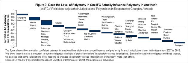
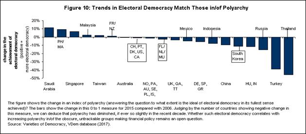
Other evidence seems to point toward polyarchy helping more competitive international financial centres than less competitive ones. Figure 9 shows the correlations between polyarchy and IFC competitiveness for specific jurisdictions. If each metropolitan financial centre reflects the polyarchy and IFC competitiveness of its host jurisdiction, Singapore and New York, in this sample, had increasingly polyartic institutions with increasingly competitive international financial centres.[96] Jurisdictions from Jakarta to Budapest had decreasingly polyartic political participation, perhaps in a bid to increase their financial centres’ competitiveness? Figure 10 bolsters such an interpretation by looking at how the achievement of electoral democracy has responded in various international financial centres in response to the global financial crisis – or visa versa.[97] Naturally, the extent of polyarchy (and possible electoral democracy) would affect the economic response to the crisis – and thus the ranking of a jurisdiction’s international financial centre.[98] Yet, as with most social economic questions, the converse might also hold. The crisis – and thus an international financial centre’s competitiveness -- affects the extent of polyarchy.[99] More participation in many cases means a replacement of incumbents, rather than an increased diversity of voices and preferences at the political bargaining table.[100] Regardless of which way causality lies, polyarchy and the size/growth of international financial centres affect each other.
The centrality of a financial centre among the flow of funds in the network of international financial centres best measures an IFC’s competitiveness. Academics have long theorised about – and even mapped -- the networks of financial capital flowing across/between international financial centres.[101] Such network maps have included measurements of financial centres’ degree of linkage, betweeness and other network statistics common to all graphs.[102] Such network measurements have allowed academics to measure things like the extent of systemic risks to the entire global banking system.[103] In such a network, geographic distance and physical centrality matters far less than network centrality.[104] Figure 11a for example shows the changes in polyarchy and changes in international financial centres’ clustering coefficients (or the extent to which a jurisdiction connects its banking partners without these other banking partners necessarily having linkages between themselves). More polyartic international financial centres cluster more with other financial centres, as measured by their clustering coefficient (basically a measure of their centrality importance in the international financial centre network).[105] Figure 11b shows the same data – fit to a non-linear curve instead of a simple line. Such a curve suggests that polyarchy increases in/for weakly and strongly clustered international financial centres. Singapore represents an increasingly important (as measured by its clustering coefficient) jurisdiction becoming more polyartic over time. Japan’s clustering coefficient rose, while polyarchy fell. The trend seems to show that polyarchy remains stable for jurisdictions losing importance over time (like Austria and Canada). Does a stable, equilibrium-level of polyarchy correspond with ever-decreasing clustering importance? Or put conversely, do some jurisdictions need to become more polyartic before they can gain network centrality?

Without controlling for other factors like macroeconomic fluctuations and the demand for capital, the network data seem to display contradictory trends. Figure 12 shows the relationship between international financial centres’ authority (or the extent to which other financial centres place money with their banks). Over the period we studied, international financial centres’ authority decreased as polyarchy in these international financial centres rose.[106] Some might argue that highly connected financial centres feel crises and other large changes in their competitiveness less – attenuating the need for the polyarchy which helps boost competitiveness.[107] Others argue that regional links have replaced global links.[108] Yet, without controlling for other factors though, these data could say anything (or nothing at all). Other factors likely interfere too badly for us to draw any conclusions about these data.
Modelling
and Operationalizing Endogenous Change in IFC Politics and Competitiveness
Changes Within and Between Countries
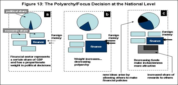
Our model focuses on
the trade-off between political rights and economic power in international
financial centres. Figure 13 shows a simplified, non-mathematical, graphical, static
version of our model. In the left-most side of the figure (part a), we depict
various sectors of the economy (as blocks) and their relative political power
as the circular pie at the top. We highlight the financial sector as the dark
blue box, whose size depends on cross-border banking liabilities (deposits and
funds from abroad). The dark blue slice of the pie represents finance’s weight
in political decision-making. In part b of the figure, we observe the financial
sector’s increased importance (share) in/of political decision making,
concomitant with its current, future, or even perceived ability to
attract capital from abroad.[109]
Such a trend might correspond with an increased focus on financial policy (and
thus decreasing polyarchy in order to implement financial policies rather than
other policies).[110]
Similar decisions in other jurisdictions negatively impact on the size of the
home jurisdiction’s financial institutions (depicted in the figure’s part c) as
a shrinking in size compared with part b. In part c, the financial sector’s political
power (concentration of influence) shrinks, yielding way to other sectors with
better/different ideas – as depicted by the black coloured slice of the
political pie. Other sectors’ inclusion in policy making increases as does
their inclusion in the economy (as shown by the larger size of non-finance
sectors).
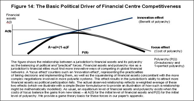
In slightly more
mathematical form, the amount of cross-border financial assets and polyarchy in
a jurisdiction depends on the focus/concentration of policy on finance and the
creation of new ideas and innovations in finance, ideas which will help attract
funds from foreign financial centres. Figure 14 shows the simplest possible
representation of these factors. In theory, more polyarchy brings more
innovation, from access to more ideas and high-powered interest in finance’s
success – as represented by an upward sloping innovation effect curve.[111]
At the same time though, more polyarchy diverts time, attention and political
capital away from finance – as shown by a decreasing focus curve. The mix
between these forces decides the level of cross-border financial system
liabilities and the level of political polyarchy – and both forces work at the
same time.
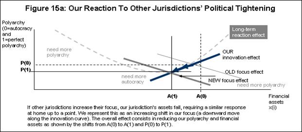
These curves allow us
to examine the impact of other jurisdictions’ changes in policy. Figure 15a
shows the effect of an increase in the focus of financial policies and politics
in one of the jurisdiction’s main counterpart jurisdictions (for example the
effect in France of the UK focusing on financial policy and Westminster’s deafening
to health and other policies).[112]
Such a policy – according to our model – would shift out the focus effect curve.
The move (and we flipped the axes to
make the figure focus on changes in financial assets) results in a decrease in
polyarchy and a fall in financial assets – as the home jurisdiction matches
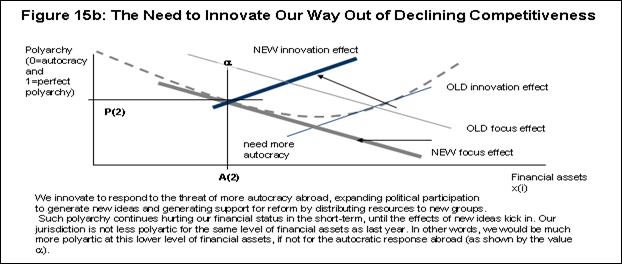
this focus and loses business to the more focused rival. Figure 15b shows the
effect at home of these changes – as local political and economic forces encourage
more participation. A shifting out of the innovation curve represents the
effect of local financiers looking for new, innovative ideas from sectors
formerly muted out, and other sectors looking for recompense for their previous
patience. Such an internal shift further undermines foreigners’ confidence in
placing their money with our financial institutions.[113]
Such a decline would have – in the past – represented the simple redistribution
of political power and economic fortunes (as shown by point a in the figure lying along the previous focus curve).
Because our counterpart jurisdictions have increased their focus on becoming
world class financial centres, we can extend our own polyarchy far less than
before in order to remain competitive... at least in this middle term.
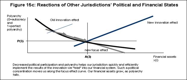
In the longer-term
though, polyarchy and financial assets held by our financial institutions
settle at an equilibrium point dictated by finance-related tastes and
technologies. Figure 15c shows the increase in financial assets and the
accompanying decrease in polyarchy from its temporary very high levels, as
financial services firms implement innovative ideas. Figure 15d shows the same
relationship between these variables as in Figure 14, though with the figure
turned on its side. The figure shows an adjustment path as other jurisdictions
change their polyarchy and/or financial assets (and thus their centrality in
the international network of financial centres). The levels A(4) and P(4)
represent those post-adjustment, equilibrium values.

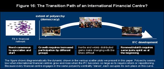
Because each wave of
innovation leads to larger, more developed financial services firms, we can
hypothesize about the way polyarchy changes as a financial centre develops.
Figure 16 shows that conjectured change. As a financial centre seeks to grow, a
pushing/guiding political force discourages dissent and encourages foreign
investment. Experiences from the UAE, Singapore, and Qatar represent the most
mediatised examples.[114]
In other cases, the lack any traditional means of economic development --
combined with a geography that gave finance a natural competitive advantage - encouraged
an autocratic political focus on finance.[115]
While many international financial centres still make finance a core area of
policy, many have started opening to other areas. To what extent does such an
opening represent a way of invigorating finance – rather than an attempt to
diversify the local/national economy? Only time will tell.
Changes over Time
In our model, international financial centres grow over time, as they focus on finance. Figure 17 shows the mental model we used to develop our model. In plate 1, we see 6 financial centres represented as a simple set of nodes. In plate 2, we show the situation where financial centre number 3 focuses on developing its financial centre. As we described in the literature review, and showed in the previous empirical overview section, such a policy-focus leads to more links and more financial assets travelling along those links.[116] As plate 3 shows, as other financial centres focus even more intensively on finance, they build out both the quantity and depth of these network links.[117] As we described in the literature review, historically one financial centre developed and grow because of growth in counterpart centres. The self-reinforcing network of financial centres grows as more and more centres decide to develop their financial centres and linkages.
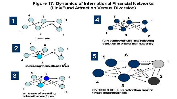
The figure shows the dynamic effects of an increase in
focus (a decrease in polyarchy) for theoretical financial centres in a
theoretical network. The light blue node (number 3) indicates an exogenous
change toward more focus. The darker blue node (number 6) indicates more
focused policies than those pursued by node 3 (simulated possibly as a random
reaction to node 3’s policy). As more nodes focus their financial policies, the
number of links increases. Plate number 4 shows the results of this race to the
bottom, where all nodes have the maximum number of links. Similarly, in plate
5, the light gray node (number 1) represents the introduction of
innovation-producing polyartic policies. The dark gray node (number 2)
represents a jurisdiction introducing more polyarchy than in node 1. The cycle
reverses itself, except such increases in polyartic policies cause links to
divert from other financial centres (preserving the total number of links in
the system). One could imagine/model an intermediary situation, where some
nodes decrease their polyarchy, while others increase such polyarchy (thus
avoiding the all-of-nothing wave-like patterns we have shown in this simple
example).
As some financial centres fall behind, they engage in the innovation needed to develop new markets, new ideas, new financial products and new markets. New innovations do not always require democracy (increased polyarchy). An increase in polyarchy does not guarantee financial innovation. Places like Singapore and Shanghai have developed for a long time without such polyarchy. In our model, such polyartic-led innovation results in a shift in financial links – a diversion of funds from other centres.[118] Polyarchy changes the relative distribution of resources – allowing for future concentration.[119] Yet, in the short-term, innovation only serves to give other financial centres time to further focus their policy priorities toward finance.
The
Data and Empirical Methods We Used
Jurisdictions, raw polyarchy and network centralities
In order to test our theories, we first had to compile the relevant data for the relevant jurisdictions.
Figures 18 provide an overview of the data we used. Figure 18a show the jurisdictions in our study, while Figure 18b shows the average values of polyarchy and eigencentrality from 2005 to 2015 – before being adjusted for the way that macroeconomic and other factors affect them. Figure 18c shows the extent to which aggregate polyarchy has changed (fallen) over the years when compares with jurisdictions’ eigencentrality. . Figure 18d shows the networks of financial relations between international financial centres in 2005 and 2015. Grouping these networks in modules, we see increasing concentration over time (matching other data).

|
Figure 18d: Financial Networks in 2005 and
2015 |
|
|
|
|
|
The figure shows
the network of cross-border bank liabilities in 2005 and 2015, sorted by the top
major groupings of financial centres. Such “modularity” (as the statistical
name for such grouping) results from closer links between module members than
the rest of the network. Such modularity changed radically over the 10 years.
In 2015, top groupings accounted for 56%, 39% and 3% respectively for the top
three modules. In 2015, the top grouping accounted for 63%, 20% and 10% of
all financial centres (with 3 more groups scoring the remainder). These
networks became thus more concentrated over time. |
|


The way that polyarchy affects the amount of cross-border liabilities that banks can attract has decreased over time. Figure 18e shows the slope of a line of best fit between polyarchy and cross-border bank liabilities placed by each jurisdiction’s largest counterpart jurisdiction. For example, in 2005, on average, a one point increase in polyarchy in any particular jurisdiction (like France) resulted in that jurisdiction’s main counterpart (like the UK) placing roughly $18 million in extra cross-border liabilities in that particular jurisdiction (France). The values in the black boxes show
the way ‘drop off’ in each jurisdiction’s counterpart’s cross-border liabilities changes for a one point increase in that jurisdiction’s polyarchy. We define such a ‘drop-off’ as the proportional difference in the value of cross-border liabilities from lower ranked jurisdiction counterparts. For example, France’s second largest counterpart jurisdiction (the US) may provide 12% fewer cross-border bank liabilities than the first ranked jurisdiction (the UK). Similarly, on average, France’s third largest counterpart jurisdiction provided 12% fewer liabilities than the US. The value in the black boxes in Figure 18e do not represent the value of such a drop-off. Instead, they measure the way that drop-off value changes as polyarchy in a jurisdiction rises.[120]
One approach to analysing our bank liabilities data might consist of looking at the ranks of cross-border bank liabilities between these financial centres. We might devise some method – like a ratio of largest to smallest counterpart jurisdiction – or some measure the deviations from the average. Figures 19 explains why we used network characteristics instead. In brief, we used network characteristics because of the dependencies between the financing partners themselves. As Figure 19a shows, the construction of any ratio of even deviation from average assumes that one observation (country’s data) do not depend on other countries. We can construct a reliable ratio (for example) if the denominator partly changes every time the denominator does. As Figure 19b shows, if we compare financial centres’ network centralities with entropies (a measure of the similarity of each partner’s bank liabilities), we see little relationship at all (as shown in the scatter plot in the lower left hand side of the figure). Figure 19c describes the term eigencentrality we use throughout this study.
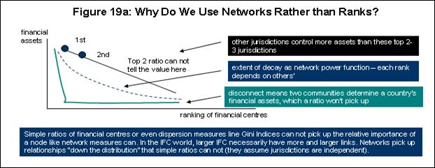

Figure 19c: What is Eigencentrality? As we describe
in the appendix, eigencentrality refers to the importance of an
international financial centre in the network of such financial centres.
Such centrality takes into account the value of cross-border bank
liabilities a jurisdiction attracts from counterpart jurisdictions. Such
centrality also takes into account the importance of that jurisdiction’s
partner countries for their own counterparts. The eigencentrality algorithm
basically traces the value of all these liabilities across the whole
network of financial centres for all jurisdictions. The most central
jurisdictions attract large amounts of cross-border liabilities from
jurisdictions which attract a large amount of these liabilities and so on
all the way through the network. The German word eigen means
characteristic (as in a physical or identifying characteristic). Such a
procedure thus finds the true or characteristic values of these
jurisdictions by already including the potential investments/liabilities
other financial centres indirectly make to that jurisdiction through its
networks of partners. Eigencentrality thus truly provides a
financial-system-wide view.

Figure 20 shows the variables we used in our study. The dependent variables consist of polyarchy in each jurisdiction as well as two measures allowing us to quantify the nature of each jurisdiction’s financial networks. In order to compare polyarchy and a jurisdiction’s centrality in international financial centre networks, we had to control for non-political factors. For example, a jurisdiction could attract large amounts of cross-border bank liabilities because of favourable exchange rates or because its government requires more funding to operate public services (and they want to use foreign funds/deposits to finance such funding).
Figure
20: List of Variables Used to Remove the Effect of Macroeconomic and Other
Variables When Estimating the Amount of Cross-Border Bank Liabilities
|
Factor |
N |
Mean |
Std.
Dev |
Min |
Max |
Diff? |
|
Dependent Variables |
|
|
|
|
|
|
|
Polyarchy |
192 |
85.06 |
12.45 |
9.21 |
94.71 |
* |
|
Largest ‘investment’ partner |
181 |
231776 |
355,563 |
1406 |
2,002,814 |
* |
|
Power Law |
181 |
-0.3 |
0.1 |
-0.63 |
-0 |
* |
|
Macro push/ pull factors |
|
|
|
|
|
|
|
Real
effective exchange rate index† |
180 |
99.03 |
7.95 |
70.9 |
125.7 |
* |
|
Real
interest rate (%) |
140 |
5.28 |
8.56 |
-10.8 |
44.6 |
|
|
Attraction Factors |
|
|
|
|
|
|
|
Market
cap. (% of GDP) |
150 |
93.94 |
61.16 |
17.57 |
282.51 |
* |
|
GDP
per capita, PPP (current thousands international $) |
192 |
37.4 |
14.56 |
4.77 |
129.34 |
* |
|
S&P
Global Equity Indices (annual % change) |
192 |
7.13 |
29.27 |
-69.94 |
125.11 |
|
|
Current
account balance (% of GDP) |
192 |
1.35 |
5.44 |
-7.51 |
31.06 |
|
|
Commercial
service exports (current billion US$) |
192 |
116.45 |
134.74 |
5.58 |
730.59 |
* |
|
Connectivity factors |
|
|
|
|
|
|
|
Air
transport, millions of passengers carried |
172 |
89.23 |
172.36 |
0.55 |
798.22 |
* |
|
Demanders of funds |
|
|
|
|
|
|
|
Central
government debt, total (% of GDP) |
160 |
60.65 |
26.52 |
18.37 |
132.36 |
* |
|
Gross
capital formation (% of GDP) |
192 |
23.07 |
4.14 |
14.73 |
43.26 |
|
|
Suppliers of funds |
|
|
|
|
|
|
|
Gross
domestic savings (% of GDP) |
192 |
26.03 |
8.08 |
12.47 |
75.54 |
* |
|
FDI,
net inflows (% of GDP) |
192 |
6.22 |
11.35 |
-5.63 |
87.44 |
* |
|
Broad
money growth (annual %) |
116 |
8.50 |
6.66 |
-25.5 |
22.05 |
|
|
Institutional factors |
|
|
|
|
|
|
|
Rule
of Law‡ |
190 |
1.35 |
0.78 |
-0.66 |
2.10 |
* |
† 100
=2010
‡
rule of law comes from the World Bank’s Governance Indicators for the variable
by that same name. All the other variables should be self-explanatory.
Diff?
refers to whether we calculated and used annual differences in this variable.
Without controlling for macroeconomic and other factors, our analysis would have been badly biased. The previous figure (Figure 20) shows the five (5) factors that we grouped these variables into.[121] Macroeconomic push-pull factors include variables that could push or pull funds across borders to a jurisdiction’s banks. Exchange rates and interest rates represent self-explanatory variables.[122] Attraction factors represent variables that might attract foreign funds (the size and performance of local stock markets, the need to finance trade, and the overall jurisdiction’s wealth/size.[123] Air transport represents our only factor measuring the jurisdiction’s connectivity.[124] Demanders of funds – like government and business investment – draw out demand for foreign funds.[125] Suppliers of local funds might help crowd out (or crowd in) foreign funds.[126] These suppliers include households and their savings, foreign direct investment and credit growth by/from the central bank.[127] Finally, no analysis is complete these days without a consideration of local institutions and the quality of regulations (as proxied by the World Bank’s Governance Indicators variable measuring the rule of law).[128]
Getting polyarchy and network centralities ready for
analysis
Macroeconomic and other factors correlate heavily with the polyarchy and centrality of international financial centres. Figure 21 shows the number of variables, combinations of these variables, and non-linearities in these variables which correlate with their jurisdiction’s polyarchy indices.[129] About 80% of all these combinations statistically significantly correlate with polyarchy at a 95% level of confidence or better. These data show that we must remove their effects before trying to find patterns related to these international financial centres’ centrality in their financial networks. Figure 22 shows the general process we used to strip away the effects of these macroeconomic variables – on both polyarchy and eigencentrality values. We regressed these variables (the covariates) on polyarchy and eigencentrality values using panel methods – in order to arrive at “pure” polyarchy and eigencentrality values.[130] As Figure 23 shows though, we had to correct the data for the interdependencies between them. The left side of the figure shows two completely independent factors (regression requires such independence to “work correctly”).[131] We see many variables clumping nearer to each other than these independent axes (known as eigenvectors). The correlation matrix on the right side of the figure further shows such interdependences between these variables. A bit fewer than half of all these variables statistically significantly correlate with each other. Without correcting for such inter-correlation, we would accidently assign part of the effect of exchange rate movements on trade balances, to cite one of the many ‘multicollinearities’ (as economists refer to such a problem) in these data.
|
|
The
figure shows the variables which statistically significantly correlate with
polyarchy across years and countries. We found these correlations using a
technique known as response surface regression. Such a technique looks for
non-linearities and interactions between variables. A computer normally could
not solve such a large system of equations. We used a particular robust
technique known as a recursive power method to find very microscopic values
of our matrix when inverting the matrix to find a solution. The techniques we
used are less important than the general message. Most of the variables in
our study statistically significantly correlate with polyarchy – interfering
with any analysis trying to spot the effects of a jurisdiction’s network
centrality on such polyarchy. We could show similar results for network
centrality – that these variables affect the extent to which financial firms
attract cross-border bank liabilities. Such multiple correlation would interfere
with any attempt to look directly at the relationship between jurisdictions’
polyarchy and network centrality. We describe below how we removed the
influence of these factors from our analysis. |


|
Figure 23: Fixing Problems That Arise When
Variables Correlate With Each Other (Multi-collinearity) |
|
|
|
|
|
The
figure shows the extent to which the covariates we try to control for correlate
with each other. Such correlation (called multi-collinearity) causes any
analysis of one variable (like government debt) to pick up the effects of
other variables like market capitalisation, trade balances, popularity as an
air travel destination and so forth.
The left part of the figure shows the relationship of our variables
with two completely independent variables (called orthogonal factors). Ideally, we need our variables to sit on
one of these axes. The right hand side shows the correlation coefficients
between the variables we used to adjust our polyarchy and network centrality
data. The coloured cells show the correlations with a 95% probability or
greater of statistically significantly varying with each other. Source:
authors calculations (with data from the Bank for International Settlements,
2017). |
|


The resulting analysis yields the ‘predicted values’ of our key variables of interest. Regressing a jurisdiction’s bank liabilities on exchange rates, government debt, air travel and other factors yields a predicted value for these liabilities. The model’s error thus reflects the part of these financial flows unexplained by these macroeconomic and other factors. We use these errors as our estimates/variables of ‘pure’ cross-border bank liabilities (after controlling for these other factors). Figure 24 provides one example of how we estimated the largest liability flow from each jurisdiction’s largest counterpart for one year (in 2005). The figure shows the actual values of these liabilities, their predicted values from our model, and the differences between the predicted values and actual values. Figure 25 shows the extent to which the values of bank liabilities for the second, third, fourth and other partner jurisdictions “drop off” (decrease in value) by rank. Such a drop off – combined with the largest finance partner – provides the new structure of financial networks.[132]
The figure shows the relationship between actual
cross-border bank liabilities from each country’s largest cross-border
counterpart and those predicted by the best fitting model. For example, in
2005, the largest value of Australia’s cross-border bank liabilities came from
the US. We estimate this predicted value for each country, for each year, in
order to estimate how funds would have flowed between international financial
centres if we could remove the effects of variables like real exchange rate
changes, GDP growth, the level of government debt, and so forth. We show a
simple linear regression here to illustrate the general idea. In practice, we
used a machine learning model (which actually did not deviate too much from
this simplistic model).

The figure shows the predicted “drop off” in the value
of bank liabilities for each of the countries in our sample. We calculate such
a drop off by sorting the value of bank liabilities coming from each
jurisdiction’s partner jurisdictions, and then fitting an exponential function
to these values. For example, the value of each of Australia’s counterpart
jurisdictions decreased by 35% when sorted from largest counterpart
jurisdiction to smallest. We show the linear predicted value of these ‘drop-off’
values in the figure to illustrate our broader methodology. We used a machine
learning algorithm to fit the actual values (though these values came pretty
close to our more complex method).
We constructed ‘pure’ financial networks for these cross-border bank liabilities by combining these new largest partner estimates with these new drop-off estimates. Figure 26 shows how we constructed these new networks – using Australia’s cross-border bank liabilities from 2005 as an example. If Australia’s largest provider of funds in 2005 held $35 million in assets (recorded on the Australian side as a liability), then our cross-country econometric estimation predicted a value of $106 million – assuming exchange rate movements, different government debt levels, and other factors had not affected these funding patterns. By rank, each counterpart jurisdiction placed 35% fewer funds with Australian banks than the one ranked ahead it. After controlling for these macroeconomic and other effects, they should have placed 29% less – in effect investing more per partner jurisdiction.

The figure shows how we adjusted one country’s
(Australia’s) cross-border bank liabilities for exchange rate movements, GDP
sizes, government debt stocks and the other factors we have previously
described. The black line shows the value of Australia’s cross-border bank
liabilities coming from its largest partner jurisdiction (the US) as roughly
US$35,000 in 2005. The next largest value of these bank liabilities came from
the UK and represented about 35% less than cross-border bank liabilities from
the US – and so forth down the line of partner jurisdictions. The predicted
value of Australia’s bank liabilities (‘removing’ the effect of all these
outside variables) came to about US$106,700 for the largest partner (again the
US), with the US and other jurisdictions’ cross-border bank liabilities’ values
decreasing by about 29% when sorted by size. Note that we used the residual of
the regression to find these values – not the predicted values themselves.
Such differences in these financial centres’ leading financial partner and the extent to which such financing drops off by rank leads to different network configurations, after going through this exercise for all the financial centres in a particular year.[133] Figure 27 shows the network of these bank liabilities in 2010, before adjusting for the effects of these macroeconomic and other variables – and after. Australia’s and South Africa’s centrality would have increased remarkably. Places like Jersey would have lost out a bit.[134] Figure 28 summarises these changes – showing the way mean values would have changed.
|
Figure 27: The Network of Cross-Border Bank
Deposits and Other Liabilities for International Financial Centres Before and
After Adjusting for Macroeconomic and Other Variables |
|
|
|
|
|
BEFORE ADJUSTMENT |
AFTER ADJUSTMENT |
|
The
figure shows the network structure (geography) of cross-border bank
liabilities for the most important international financial centres for 2010
(as one example from 2005 to 2015). For negative values of these flows, we
switched the direction of these flows, from destination to source (rather
than the other way around). We calculated each country’s eigencentrality from
networks like these for each year from 2005 to 2015. These eigencentralities
measure the importance of an international financial centre, taking into
account the size of cross-border bank liabilities its counterpart
jurisdictions attract from their own partner jurisdictions. The final
eigencentralities thus exclude the effects of macroeconomic and other factors
we used in our preliminary regressions. |
|


Figure
28: Summary Statistics for Polyarchies and Eigencentralities Used in Study
|
Variable |
Valid N |
Mean |
Minimum |
Maximum |
Std.Dev. |
|
Pure Polyarchy |
160 |
18.81 |
0.0 |
119.38 |
11.15 |
|
Difference in Pure Polyarchy |
141 |
0.74 |
-7.5 |
45.51 |
5.27 |
|
Voice |
192 |
114.83 |
-170.0 |
173.96 |
55.87 |
|
Difference in Voice |
163 |
-2.05 |
-162.3 |
91.89 |
19.48 |
|
Old eigencentrality |
128 |
90.79 |
0.0 |
100.00 |
11.97 |
|
New eigencentrality |
156 |
37.80 |
8.7 |
100.00 |
33.28 |
|
Change in new eigencentrality* |
130 |
63.68 |
-10000.0 |
10000.00 |
3646.91 |
|
Invest Entropic Measure * 100 |
184 |
15.91 |
6.7 |
54.26 |
8.56 |
The figure shows
the differences in the values of our variables, before and after controlling
for outside factors. “Pure” variables refer to variables calculated as the
‘error’ or residual of the regression analysis we described earlier, adjusting
for the effects of macroeconomic and other factors. We provide data for voice and entropy, two
variables which we will discuss in more detail as we test the robustness of our
analysis.
* We rescaled
these changes to maintain the same scale as the other data.
Changes over time
Even after finding the “pure” values of polyarchy and eigencentralities, we still need to make sure that any correlation between these variables does not arise from inertia. If a country’s polyarchy in any year depends mostly on such polyarchy in the previous year (or years) before, then such a dependence on the past can block out any attempt to correlate such polyarchy with the network importance of the jurisdiction and its partner/competitor jurisdictions. Figure 29 shows the extent of such inertia – which economists call auto-correlation – for select jurisdictions’ eigencentrality and polyarchy. We observe no value approaches one (1) – the value at which last year’s polyarchy equals this year’s polyarchy.[135]
We can then look at how each country’s polyarchy-eigencentrality adjusted over the decade. Figure 30 shows some examples of our data. The left hand side of the figure shows Australia’s polyarchy compared with its own eigencentrality. We observe a hill-like pattern in this one example of Australia’s polyarchy compared with the jurisdiction’s own eigencentrality.[136] Australia’s eigencentrality and polyarchy have risen together for lower levels of the country’s eigencentrality. As Australia gains prominence in global international networks, polyarchy fell. We similarly show one example of the way Australia’s polyarchy changed as Denmark’s eigencentrality changed in the right part of the figure. In this particular outcome, Australia’s polyarchy increased as Denmark eigencentrality rose. The trend on the bottom of the figure shows the way that Australia’s polyarchy responded to a change in its eigencentrality – for various levels of its eigencentrality. Such a figure – called a ‘spider plot’ – shows the way that polyarchy reacts to a jurisdiction’s eigencentrality over all possible states of these variables.
The “spider” graph in the last part of the figure shows a similar trend – adjusting for the randomness of these variables. Namely, this spider graph shows the results over 1,000 simulations – ensuring that the final relationship roughly depicts the relationship without very wide confidence intervals leading away from this line. Yet, this method of analysis treats different observations from different years as random draws from a deeper relationship between these two variables. Such a procedure gives a snapshot picture, by using data collected over time.
|
Figure 30: The Relationships Between Polyarchy
and Eigencentrality (Actual and Bayesian) |
|
|
|
|
|
|
|
|
The figure shows
the relationship between Australia’s polyarchy and eigencentrality from 2005
to 2015 as an example of the methods we used in this study. The top left
panel shows a simple correlation of these variables for Australia. The top
right panel shows the simple actual correlation between Australia’s polyarchy
and Denmark’s eigencentrality. The bottom curve – called a spider plot –
shows the conditional mean of the way Australia’s polyarchy changed for
changes in its eigencentrality, over various levels of such eigencentrality.
In this figure, changes in Australian polyarchy, compared with changes in
eigencentrality rose when Australia did not occupy too central a position in
global financial networks (ie possessed low eigencentrality). Such polyarchy
increases the slowest at medium levels of eigencentrality – supporting the
model we presented in the previous section of our paper. The figure shows the
relationship over 1,000 simulations – and does not change when we rerun the
simulations (namely we have a consistent parameter). Think of the figure as
fitting regression lines on polyarchy and eigencentrality when dividing
eigencentrality into sub-samples by size.
|
|


We should explain further the importance of the spider plot. If the top part of Figure 30 shows one realisation of the way Australia’s polyarchy changed as the jurisdiction’s eigencentrality changed from 2005 to 2015, we could imagine “alternate universes.” We could imagine these data come from distributions which we can not see. We saw these data – but we could have easily seen other data too. The spider plot presents a Bayesian analysis of these variables. We resampled randomly 1,000 times from the historical data and the likely distribution generating these data.[137]
Over all these samples, we obtained the stable relationship between the way polyarchy changes compared with eigencentrality – for various levels of eigencentrality. Such analysis allows us to see how polyarchy might change its response, as eigencentrality changes. We could (and do!) conduct similar analyses for all pairs of polyarchy and eigencentrality between international financial centres – providing a detailed map of political change in response to financial competitiveness.
What about adjustment over time? Polyarchy must respond to different eigencentralities – both the jurisdiction’s own eigencentrality, as well as the centrality of its partner/competitor jurisdictions. Figure 31 shows the way we can differentiate between these effects, using a type of analysis known as Fourier Spectral Analysis. Such an analysis looks for wave patterns in each dataset. Longer waves mean an effect takes longer to appear. Looking at France’s reaction to the increasing eigencentrality for the jurisdictions shown in the figure, we see that polyarchy responds most in the short-term (in 1 to 2 years). After that, polyarchy responds very minutely. France’s polyarchy responds more to Australia’s increased competitiveness (as measured by increased eigencentrality) than to the other jurisdictions – making Australia somehow a more important rival for France – even if French politicians and financiers do not recognise Australia as such a rival. By tracking the extent of these changes over time, we can observe how our detailed map of political change in response to financial competitiveness changes over time.
 How does the polyarchy of a country (in this case France) react to the
increasing centrality of partners’/competitors’ financial centres over the
years (from 2005 to 2015)? The figure shows the way that way that French
polyarchy ‘correlated’ with changes in the eigencentrality of the jurisdictions
shown in the figure for the same period. Such a correlation changes with time.
We show the short-term, middle term and long-term reactions as a 2 year, 2.5
year, 3.33 year, 5 year and 10 year reaction to changes in these
eigencentralities. Unlike an impulse response curve (which looks at the effects
over time of a single, sudden shock like a one-time change in such
eigencentrality), these curves show the periodic reaction (for example the
longer term 5 year effect separating out the 2 year effects on their own). The
equations in the figure show the decline in response from these 2 year to 10
year reactions as a function of time.
The R2 shows how well our estimated decline in response over time
matches the data (with 100% representing perfect matching and 0% representing
no match at all). This analysis can detect changes in causality (namely
whether polyarchy responds to – or actually causes – changes in eigencentrality
of other financial centres. Specifically, we look at the ‘gain’ in a
bivariate Fourier time series analysis for the periods shown, with ‘coherency’
of each period provided the R2s we report in the figure.
How does the polyarchy of a country (in this case France) react to the
increasing centrality of partners’/competitors’ financial centres over the
years (from 2005 to 2015)? The figure shows the way that way that French
polyarchy ‘correlated’ with changes in the eigencentrality of the jurisdictions
shown in the figure for the same period. Such a correlation changes with time.
We show the short-term, middle term and long-term reactions as a 2 year, 2.5
year, 3.33 year, 5 year and 10 year reaction to changes in these
eigencentralities. Unlike an impulse response curve (which looks at the effects
over time of a single, sudden shock like a one-time change in such
eigencentrality), these curves show the periodic reaction (for example the
longer term 5 year effect separating out the 2 year effects on their own). The
equations in the figure show the decline in response from these 2 year to 10
year reactions as a function of time.
The R2 shows how well our estimated decline in response over time
matches the data (with 100% representing perfect matching and 0% representing
no match at all). This analysis can detect changes in causality (namely
whether polyarchy responds to – or actually causes – changes in eigencentrality
of other financial centres. Specifically, we look at the ‘gain’ in a
bivariate Fourier time series analysis for the periods shown, with ‘coherency’
of each period provided the R2s we report in the figure.
Does
Polyarchy React to a Financial Centre’s Centrality?
Before analysing our main research question, we should ask what effect did changes in polyarchy in one financial centre have in/on other financial centres? Figure 32 shows the correlations between the polyarchies of several of the countries we studied. In all cases, except one, polyarchy in one jurisdiction met with more inclusiveness in other jurisdictions – after adjusting for numerous factors and trends that could have affected these countries simultaneously. By removing these outside effects, we could be increasingly sure that financial centres reacted to each other – rather than international macroeconomic changes which would have caused all these jurisdictions’ politicians and financial elites to restrict (or not) polyarchy. About half of these jurisdictions exhibited statistically significant correlations – for a level of statistical significance when we should only expect to observe about 5% of these polyarchies to have statistically significant correlations with each other.
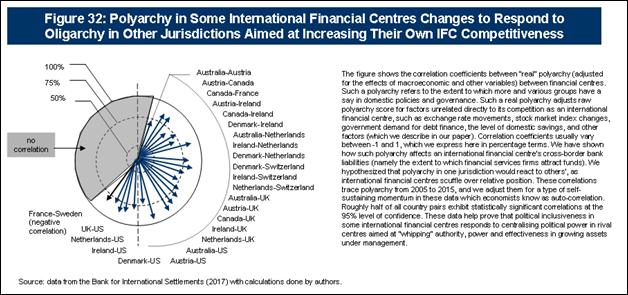
How do we know these correlations actually represent something more than just random chance? Maybe we could collect data from these countries 10 years from now, and see a different pattern? Figure 33 shows the correlation between countries’ polyarchy if we could draw data from 1,000 “alternate universes.” Namely, we fit a pattern to all these countries’ polyarchies and simulated the same variability and correlation structure in polyarchy that these data actually exhibited from 2005 to 2015. We see that, for all countries in our study, the correlation between one country’s polyarchy and another’s comes to about 0.25 on a scale ranging from -1 to 1. In other words, changes in a country’s polyarchy ‘explains’ or ‘accounts for’ about 25% of its peer countries’ polyarchy. Even a sceptic must accept that the polyarchy of one financial centre affects others.
Figure 33: Changes in the Polyarchy of Other Financial Centres
Explains about 25% of a Jurisdiction’s Own Change
(Bayesian Approach)
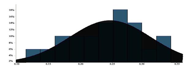
The figure shows the distribution of correlation
coefficients across all pairs of financial centres’ polyarchy scores in our
study. We calculated this Bayesian statistic as follows. First, we fit
an auto-regressive model to polyarchy in both jurisdictions of each of 54 pairs
of countries, simulating what other possible evolutions of these polyarchy
scores could have happened over a 10 year period. We then calculated, for each
pair, a correlation coefficient – which changed randomly according to the
random variation measured in the auto-regression of each pair of polyarchies.
We then averaged all of these correlation coefficients to arrive at a single
average correlation. Finally, we simulated 1,000 alternative 10 year periods –
arriving at one average correlation coefficient across all pairs of countries
for each of the 1,000 alternative periods. We show the distribution of these
1,000 averages (a Normal distribution centred at 0.25 and with a standard
deviation of 0.06) as the black bell curve. We show a random sample of 44 of
these averages as the blue bars just to see how one particular draw might look
like. The Normal Distribution actually scored highest on the Akaike Information
Criterion which helps statisticians decide which distribution best fits the
data. The main message from the figure
is that these data must be correlated (the alternative of ‘no correlation’ has
less than a 0.01% likelihood of being true).
How exactly does such polyarchy flow through the international financial centre networks? We do not show the results of all the simulations we ran – simulations which attempt to track which jurisdictions account for more or less influence overall. Yet, we show the outlines of such influence in Figure 34. The figure shows the correlation between polyarchies for the jurisdictions we studied, with larger nodes representing those jurisdictions with larger overall correlations of their polyarchy with those of other financial centres. The left part of the figure shows one of these correlations before using eigencentralities to see how the correlations between the correlations of various financial centres’ polyarchy work themselves out.[138] Looking only at correlations as links with a ‘weighted degree’, we observe the US having a relatively low correlation with other financial centres (remember the correlation we show appears at random from a fixed distribution and other correlations may vary a bit from this one).[139] Even though the US’s correlation came out relatively low in this first simulation, we see that – after accounting for all these correlations and having correlations in polyarchy “work their way out” through the network; the US’s polyarchy again correlates highly with other jurisdictions (as shown on the right side of the figure). The difference between the left-hand side and the right-hand side of the upper part of the figure thus give us an idea about how changes in polyarchy ripple through to the US (and changes in the US to ripple outward). In the lower part of the figure, we show a second simulation; showing a higher correlation for the US with other jurisdictions – a correlation which remained high after accounting for the way such influence flows across the network. Some countries will change their correlations from simulation to simulation (depending on the strength of the original correlations with their peers). Yet, some jurisdictions will predominantly account for the overall 25% correlation coefficient between jurisdictions which we described in the previous figure.
|
Figure 34: The US Becomes More Polycratic as a
Polyarchy “Wave” Moves its Way Through the International Financial Network |
|
|
|
|
|
Weighted
degree for simulation 1 |
Eigencentralities
for simulation 1 |
|
|
|
|
Weighted
degree for simulation 2 |
Eigencentralities
for simulation 2 |
|
The figure shows
correlation coefficients for each international financial centre in our study
represented as a network. Higher correlations with other jurisdictions make a
jurisdiction’s node size bigger (and link colour darker). As such, these
links to not represent actual flows per se...but correlations. The
graphs of the left side of the figure shows two of the correlation
coefficients resulting from our simulation (which itself comes from
correlation data between these jurisdictions). The graphs on the right show
the correlations after “running through” the network – taking the correlation
of partners’ correlations into account (eigenvalues). These correlations
change from simulation to simulation. Yet, some patterns – like the US’s high
correlation – remain a relative constant across simulations. |
|


How does polyarchy adjust to changes in other financial centres’ eigencentrality? Figure 35 shows the conditional distribution between these two variables. In other words, how do changes at low levels of eigencentrality – versus high levels -- affect changes in polyarchy? For all countries, higher eigencentrality levels corresponds to lower levels of polyarchy. Looking that the way polyarchy changes to eigencentrality, as a percent of eigencentrality itself, we see a different relationship. Polyarchy drops most quickly at small levels of eigencentrality. Presumably, rivals need to adjust their polyarchy quickly, before growing international financial centres become a too much a threat.
|
Figure 35: Polyarchy Decreases as Rivals Become More Central to/in Financial Networks |
|
|
|
The figure shows
the way that polyarchy in international financial centres changed as their
partners’ eigencentralities changed. Such a graph depicts a conditional
distribution – the distribution of polyarchy for every level of partners’
eigencentrality. Polyarchy falls across international financial centres as
their peers’/rivals’ eigencentralities rise. The blue lines show the results
of several resampling rounds. The black lines show the distribution of the
quotient of polyarchy and eigencentrality as the dependent variable (thus
removing the effect of eigencentrality ‘size effects’). |

Where do we see the “innovation effect” in our data? According to our model, we would expect financial centres to start innovating when rivals become very large. Yet, in the data above, we see only a negative reaction to rivals’ growth. Namely, polyarchy always seems to shrink – no matter how big rivals grow. To find such an effect, we must look at the way international financial centres’ polyarchy responds to their own centrality – logical, as all “politics is local” (to coin the phrase).[140]
Polyarchy (and thus possibly innovation) increases as a jurisdiction’s own eigencentrality rises –though not for every financial centre. Figure 36 shows the same conditional probabilities of a high or low polyarchy score for low or high eigencentrality values in/of a jurisdiction. We see that, for countries like Ireland and Sweden, polyarchy rose quickly as these jurisdictions’ own eigencentrality rose over time. In cases like the US and Switzerland, polyarchy fell slightly. Figure 37 shows these relationships more clearly. In that figure, we plot the first three years’ polyarchy and the final three years’ average as a percent of the 10 year average. We show which countries’ polyarchy scores rose as their own eigencentrality rose – versus those jurisdictions that fell. Because these trends come from 1,000 simulations based on our data, we can reliably conclude that these patterns do not simply represent an accident of history (or one outcome among many). Bayesian estimation allows us to present data “robust” to any particular case or situation.
Figure 36. Own Responses to Own Eigencentrality

The figure shows the polyarchy of jurisdictions as
their eigencentrality varies across time. When more central to international
financial networks, many jurisdiction’s polyarchy rose – exhibiting the
“innovation” effect we hypothesized in our model. Yet, not every jurisdiction
displayed this pattern. Some reasons for the lack of such a response may
include our short time period (only 10 years), bad data on polyarchy, our model
is wrong or at least wrong for some jurisdictions.
Figure 37: Some Countries Became More Polyartic as their own
Eigencentrality Rose
The figure shows the change in polyarchy for
increasingly higher levels of eigencentrality. We first looked at the
correlation between each jurisdiction’s own polyarchy and eigencentrality. Next
we simulated 1,000 times changes along the distributions defining these scores
to arrive at a conditional distribution for polyarchy (conditional on
eigencentrality) – as shown in the figure above. To calculate these changes, we
took the average scores for the first 3 years and last 3 years of the decade
long series. We divided these scores by the decade average and multiplied by
100. The resulting Bayesian values show the way these financial centres’
polyarchy changes with their own eigencentrality.
To sum up our analysis, we have found support for our model of democratic (polyartic) change in international financial centres. While we “cheated” – by relying on decades of experience and various studies pointing to the roles of polyarchy and financial network centrality, no one has tested such a relationship using quantitative methods before. We found that jurisdictions use polyarchy (and politics more generally) as a method of developing their own international financial centres – and to react to the development of other financial centres in the international financial centre network. We found that a jurisdiction’s own development causes polyartic change in large financial centres more often than foreign centres – likely a response to remain competitive.
How
Reliable Are These Results?
How reliable are our results? One way to assess the quality of our study consists of comparing our results with those obtainable by other/ordinary methods. For most studies like this, standard practice consists of running regressions (or some variation of regression) to see if eigencentrality correlates statistically significantly with polyarchy. We ran a normal series (or panel) of panel regressions – dividing models into several types.[141] Figure 38a shows the results of these regressions. “Old” eigencentrality refers to the eigencentralities we obtained, before removing the influence of any other variables. In theory, this regression would result in the same relationship between polyarchy and eigencentrality we found earlier – as regression treats each variable separately (independently). Yet, we see that the parameter telling us how much jurisdictions’ eigencentralities affected their polyarchy could swing about wildly – depending on the model. Such a model, overall, describes most of the variation in polyarchy (as shown by the R2 statistic).[142] Yet, even after controlling for time and country-specific effects, regression can not even distinguish whether a positive or negative relationship exists between eigencentrality and polyarchy.
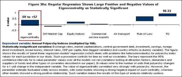
What about our decision to use eigencentralities instead of bank liabilities directly as a measure of financial centres’ importance in global financial centre networks? We previously explained the philosophical reasons for using centrality, instead of bank liabilities directly. Figure 38b shows a practical reason why using these flows would not have helped. Polyarchy positively correlates with these bank liabilities (namely those from each jurisdiction’s largest counterpart). Yet, even after controlling for other factors, the overall model performs poorly – as measured by R-squared. The large uncertainty around our estimate of polyarchy’s influence on such liabilities further shows how poorly such regression models would work.
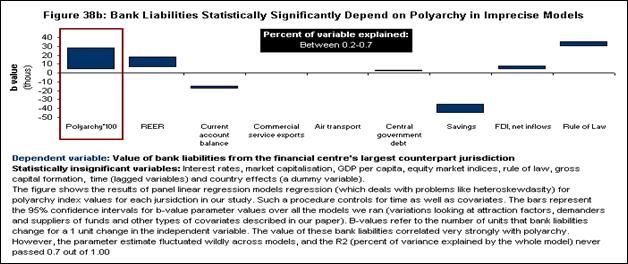
Maybe if we looked at rates of change – instead of levels – our regression models would perform better? Because of the impact of time (and the influence of both variables’ pasts and other factors we do not observe), most econometricians regress rates of change. Figure 38c shows the effects of such a regression. We look at changes in our other variables for consistency (ie looking at the change in market capitalisation over one year). Eigencentralities have a positive relationship with the way polyarchy changes in particular jurisdictions; though, not very much – again as judged by the uncertainty/low value of eigencentrality and the R2. Unfortunately, simply differencing our variables wouldn’t fix this analysis.

Maybe we used the wrong variables? Perhaps other measures for such political inclusion, such as the World Bank’s “voice” variable, would perform better? Figure 38d shows the results of regressions looking at the relationship between voice (as one example of such a variable) and polyarchy. We see a positive correlation (suggesting substituting polyarchy for a similar measure would lead to similar results). Unfortunately, without adjusting polyarchy for the influence of other variables, polyarchy has no predictive power in explaining differences in bank liabilities from an international financial centre’s counterpart jurisdictions (we describe such differences as the exponential drop-off in such liabilities and explain what we mean by this above and also in our methods section). We could do the same analysis using different measures of centrality (and we calculated all these jurisdictions’ authority and hub values, Pagerank value and clustering coefficient.[143] In all these cases, the high correlation between these variables leads to the same conclusions. Simply swapping out our variables for others probably would not change our results.

Maybe we should have used other measures of financial centre’s success – like the sale (or even purchase) of equities, short-term and long-term debt from its peer international financial centres? Figure 39 shows why we can not use securities trading as a measure of financial centres’ success. For Australia in 2015, we see only five jurisdictions make-up more than 90% of its securities’ buyers. Among those centres, we see a seeming specialisation between financial centres’ purchases of Australian stocks (US and UK as major buyers), rather than long-term bonds (with Japan as a major buyer). But so what? What do we learn by finding out that very polyartic jurisdictions buy more equities than debt (for example)? Such an exercise would waste time, and provide little insight into our question.
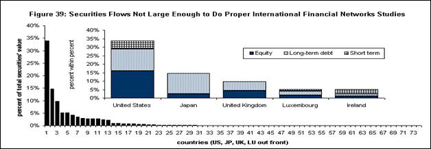
What about typical time series methods – like vector auto-regression and auto-regression/moving average methods? Could we have found better or more parsimonious explanations using these popular methods? Figure 40 shows the outcome of vector-autoregression for the annual average values of eigencentrality and polyarchy, averaged across countries for each year. Even this simple model predicts that polyarchy falls as eigencentrality falls over time. Such a method shows us what we already have seen (polyarchy fell across time for the jurisdictions we studied). Eigencentrality correlates with this falling polyarchy, so naturally time series methods would find a similar pattern (particularly as vector auto-regression and similar methods do not control for outside variables as we do). Again, these methods lead nowhere – possible explaining why so few people have researched this question.

A final objection might state that financial institutions operate in places far removed from their host countries. Just because the Cayman Islands attract large amounts of cross-border bank liabilities, does not mean its companies ultimately profit. A financial institution’s nationality and residency can differ greatly from its location (which our data track). For example, the US investment house Morgan Stanley can incorporate a British Virgin Islands holding corporation to operate in Hong Kong. Whose polyarchy is important in a case like this? Figure 41 shows the extent to which financial institutions’ nationalities (and thus the possibly likely final destination of funds ultimately repatriated to them) differ from locations and residencies. Effective advantage refers to a jurisdiction’s ability to attract more funds from foreign banks than their own banks can attract. Clearly – barring large geopolitical events - polyarchy in the British Virgin Islands would not affect a French bank differently than a US one.[144] Maybe Switzerland’s high polyarchy gives its nationals an advantage in foreign locales? If that were true, then China (the next largest beneficiary of the “nationality effects” reported in the figure) should have similar levels of polyarchy. Mexico’s polyarchy does not encourage companies to incorporate there, and then operate in South America (for example).[145] Mexico’s effective advantage clearly depends on polyarchy effects at home. Polyarchy works on a territorial basis.
Figure 41: Whose Jurisdiction’s Banks Rely More on Economic Clout
Rather Than Their Nationality in Cross Border Finance?
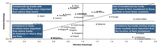
Figure
41 Continued: Jurisdictions Ranked by Ratios of Effective Advantage to Nominal
Advantage
|
Jurisdictions
With Net EFFECTIVE Advantage |
||||||||||||
|
Bermuda |
7.28 |
Cayman Islands |
1.72 |
Hong Kong |
0.54 |
Portugal |
0.14 |
|||||
|
Indonesia |
6.36 |
Luxembourg |
1.59 |
Singapore |
0.54 |
Belgium |
0.14 |
|||||
|
Mexico |
5.51 |
Ireland |
1.43 |
Brazil |
0.51 |
South Korea |
0.07 |
|||||
|
Turkey |
3.45 |
Panama |
1.10 |
Bahamas |
0.50 |
Bahrain |
0.05 |
|||||
|
Cyprus |
2.84 |
Finland |
0.69 |
Malaysia |
0.36 |
Austria |
0.05 |
|||||
|
Chile |
2.35 |
United States |
0.59 |
United Kingdom |
0.24 |
India |
0.01 |
|||||
|
Jurisdictions
With Net NOMINAL Advantage |
||||||||||||
|
Switzerland |
-1.46 |
Japan |
-0.90 |
Taiwan |
-0.51 |
Italy |
-0.34 |
|||||
|
China |
-0.98 |
Germany |
-0.65 |
Netherlands |
-0.49 |
Denmark |
-0.32 |
|||||
|
Sweden |
-0.92 |
France |
-0.63 |
Spain |
-0.44 |
Australia |
-0.26 |
|||||
|
Canada |
-0.90 |
Greece |
-0.56 |
South Africa |
-0.37 |
|
|
|||||
The figure shows
the extent to which the value of a jurisdiction’s cross-border banks’ claims
based on residence and/or nationality exceed the value based on location. In
other words, rather than looking at where a bank physically invests abroad
(location), we look at the “nominal” nationality of that bank (where the bank
is legally registered) and its “effective” nationality (where it does the most
business). We calculate these figures by taking the cross-border claims in
2016’s last quarter and finding the ratio of banks’ claims defined by these
banks’ main jurisdiction of business and location, as well as the ratio claims
for banks defined by these banks’ nationality and location. Thus, we might
measure the investments of a French bank (defined by nationality), with most of
its business done in Luxembourg (defined as residence) located in Canada
(location). A ratio of one (1) for France would mean that the value of French
cross-border investments by nationality would equal the value of investments
made in France. In the graph above, we note those jurisdictions with ratios
less than one – indicating that “value” of location exceed the value of
investments defined by banks’ nationality or principal place of business. The
table below the graph subtracts these two ratios (value of banks’ assets
defined by the nationality of the bank and the location of investment as the
first ratio and the value of banks’ assets defined by the principal market of
the bank and the location of investment as the second ratio). Such a difference
gives the extent to which each jurisdiction serves as a principal place of
investment for banks world-wide compared with national identification of a
bank.
Source: Bank for
International Settlements (BIS) Locational Banking Statistics database.
In summary, standard methods of econometrics seem very unlikely to produce the kind of analyses we have done. To the extent they are able, these other methods support of findings. Without adjusting polyarchy and/or bank liabilities for macroeconomic and other variables, any analysis of our research question would likely contain serious errors. Even with these adjustments, and by using Bayesian methods, we have at least constructed an argument for polyarchy’s role in international financial centre competitiveness.
Conclusion
International financial centres like Doha, Dubai, Shanghai, and even more recently Moscow and Istanbul, seem to show that limits on national and/or local democracy help promote financial centre growth. New York and London, the world’s two leading international financial centres, sit in relatively democratic jurisdictions. Yet, even historians could argue that their growth came from government/political support – not from freely democratic, autonomous development. What do the data say?
In this paper, we have looked at the role of polyarchy (and thus increased democracy) in aiding the development of an international financial centre. We find support for decades of theorising that financial centres’ rely on increased autocracy (less polyarchy) to help grow out their financial centres. Yet, these results do not support more autocratic (or even authoritarian!) government. The successful international financial centres of today limited polyarchy in the past (if even ever so slightly) in order to help grow out their financial centres.[146] Yet, they also enfranchised other groups in their polyarchy to generate political support for the financial centre, bring in new ideas and financial innovations, and balance out national economic growth. These financial centres’ policymakers restricted and expanded polyarchy (either intentionally or unintentionally) to grow their financial centres.[147]
At the heart of our methodology lies the comparison of polyarchy and a financial centre’s centrality in the international network of financial centres. We looked at the growth of these financial centres as the extent to which they attracted more funds from abroad (specifically cross-border bank liabilities). We looked at their centrality by computing network graphs and calculating a robust form of such centrality known as ‘eigencentrality.’ We found that polyarchy decreases as other international financial centres’ centrality in the global financial centre network expands. Such polyarchy – when used by some very central jurisdictions to remain central – “spreads.” And despite the evidence from the last 10 years, our model predicts that polyarchy should increase in many jurisdictions over time because financial centres rely on increasingly polyartic governance as a way to foster financial innovation through increased participation by non-previously powerful sectors. Yet, growth in an international financial centre’s centrality in global financial networks relies – in the shorter term -- on tapering polyarchy. Decreases in polyarchy have probably helped financial centres get ahead, depending on the centre and the time.
Our results inform several debates of the day. Activists for or against Britian’s exit from the European Union (Brexit) or Hong Kong’s total reunification with China in 2047 and others praise or condemn the effects of polyartic government on their financial centres’ performance. Yet, before our study, they had little empirical evidence for doing so. Our study suggests that they should try to choose a level of democracy or polyarchy which maximises the performance of their financial centre overall. Instead, they should worry about when polyarchy changes vis-a-vis other financial centres. The mixed equilibrium our model predicts – namely that successful financial centres should adjust their polyarchy counter-cyclically with other centres – means that no level of polyarchy will always be best for a financial centre. Hong Kong’s success as an international financial centre – like Britain’s – will depend on whether they restrict or expand polyarchy at the right time in response to other financial centres. Little surprise there.
Appendix
I: A Model of Domestic Political Change and a Model of Network Change
The micro-foundations of financial assets versus polyarchy
We start our model with a game played between government and banks. Figure A1 shows the set-up for this game. We assume each financial centre i (or wannabe financial centre) has a government able to supply some level of polyarchy P. Let’s start with a level P(0). Let’s imagine the government may supply a bit more or a bit less polyarchy (labelled in the figure A1 as ‘up’ and ‘down’ respectively). As we have already described in detail in our main paper, more polyarchy reduces banks’ profits due to a distracted policy agenda less able to focus on the best financial policies, less policy coherence and likely instability. If we use a representative bank to replace the all banks in a jurisdiction, then equation (1) shows the way that more polyarchy affects the value of foreign assets on the local jurisdiction’s banks’ profitability. Polyarchy affects these assets through a parameter f which affects the marginal size of polyarchy’s effect on these assets. The parameter l describes the banks’ specific ability to turn these policies into profits. We set the profits and costs at a numeraire of 1 to avoid complexity.[148] Equation (2) gives the return to these banks as a fraction of change in foreign assets.
![]() for
for ![]()
![]() and
and ![]() (1)
(1)
![]() and
and  (2)
(2)
If we allow two symmetric countries to compete for these assets, then the foreign bank profits r* depend on P*(j) such that f*<f if j*<j. In other words, the jurisdiction with the lower polyarchy, in this local setting, wins more foreign assets.

The government plays a similar game, though in reverse. As equation (3) shows, the amount of political capital governments earn (and want to maximise) comes to Ki for each financial centre’s i governments. More polyarchy increases the government’s political capital directly (through a parameter b) and indirectly through its banking constituencies (their political power d which rises as a function of their foreign assets under management A. Remember though that these assets fall with increasing amounts of polyarchy (at least in this short-term local setting). If welfare W represents the changes in this political capital, then equation (4) describes the sum of such welfare. The optimal condition clearly obtains when W = R, as described by equation (5). After some manipulating, equation (6) shows the best level of assets for a country. With some slight rearranging, the second part of equation (6) shows the optimal amount of polyarchy. In theory, we can simply replace the words “innovation effect” in Figure 14 with the words “political capital” effect, and still have derived a sufficiently grounded model for our purposes. However, we want something more game-theoretical.
![]() for
for ![]()
![]() and
and ![]() (3)
(3)
![]() (4)
(4)
![]() =
= ![]() (5)
(5)
 and
and ![]() (6)
(6)
The additional game theoretic element to our model comes in through the innovation effects we have not yet modelled. To start off this part of the analysis, let’s imagine desired outputs of our game – as we show in Figure A2. Government tries to maximise its political capital. Financial institutions want to maximise assets under management. The foreign investors – that we have assumed simply take the highest returns (until now) – also want a certain degree of stability. We need one of these players to demand less polyarchy (investors) in order to more simply balance out the demand for more polyarchy from financial firms looking for innovations. Let’s make innovation I a simple decreasing function of polyarchy and an increasing proportion of time t, while w is the extent to which innovation ‘accumulates’ in an account when polyarchy rises. The more polyarchy – and the longer polyarchy stays down – the more potential innovation the jurisdiction has to “spend.” If I=Pwt, then let’s set A=Iy in order to make such asset accumulation a simple function of such innovation, and thus A=P(wt)/y.
![]() and
and  (7)
(7)

Foreign investors’ love of stability represents the last (though actually unused part) of our model. Let’s further imagine that foreign investors feel more stable (with S as a some kind of “stock” of stable feelings like animal feelings) as polyarchy decreases in the countries they invest in. If r represents the increasing instability they feel as they put more assets into a country with a certain level of polyarchy, then S=Pexp(-rA). But just setting the derivative equal to this instability parameter gives us equation (8) – a short-cut to sure. However, as we do not use these equations in simulations or in applied work, we allow ourselves to take this simplifying short-cut. With this equation, we have defined all four stock levels of our model – political capital and assets which we use in this model and innovation and stability which remain running in the backgroud (and which future scholars may wish to theorise further).
![]() (8)
(8)
Supply and demand for polyarchy, innovation and investment assets
With the micro-foundations for the supply and demand for investment assets and polyarchy in place, we can define the supply and demand for these variables. Figure A3 traces the argument for demand for polyarchy in our model. From the interaction in the network of international financial centres, we can imagine an “exogenous” demand for innovation and stability (which we make endogenous for now to make our argument easier to follow). Our foreign investors respond mechanically to the trade-off between innovation and stability -- as defined in equation (8)). The bank in local jurisdiction, facing this level of demand for polyarchy, communicates this level to the government. Government then looks at the demand for polyarchy from its constituencies, and decides on a level of polyarchy which maximises its welfare – as we have stated in equations (1) and (3) representing demand by banks and government constituencies respectively. As Figure A4 shows, the government responds with a ‘supply’ of polyarchy – ranging from somewhere between perfect autocracy and perfect democracy. As we described in Figure A2, higher polyarchy (for example) may reduce financial firms’ competitiveness and thus r. Yet, these firms’ ‘innovation account’ rises, allowing them to draw on such innovation to increase assets when costs/benefits shift in the global financial network.
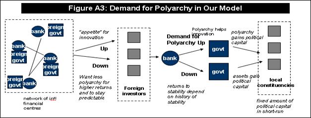

The supply and demand for polyarchy in each
jurisdiction thus balance each other for every jurisdiction. Figure A5 shows
how we move from a game based on sets of actors, to a continuous decision by
each game player. The government response of more polyarchy has two effects on
financial firms. First, they lose assets by having a lower profitability r
for higher levels of polyarchy (as shown by the downward curve marked ‘focus
effect’). Second, they gain assets, to the extent they have saved up a stock of
innovation I, which only increases as polyarchy increases. Naturally,
the trade-off between these two effects depends on the parameters we have
described in the model above. Yet, the joint effect results in the level![]() and P(j) which we defined in equation (6). Instead of
assuming j ‘states’ of increasing and decreasing polyarchy, we can make j
a continuous input – thus making P also a continuous variable. The
formulae do not change in the move from discrete sets of policies to a
continuous range of polyarchies.
and P(j) which we defined in equation (6). Instead of
assuming j ‘states’ of increasing and decreasing polyarchy, we can make j
a continuous input – thus making P also a continuous variable. The
formulae do not change in the move from discrete sets of policies to a
continuous range of polyarchies.
How do we draw out the asset curve in bold and separate out the two effects into focus and innovation effects respectively? Equation (9) shows the effects of differentiating the first part of equation (6) by polyarchy’s effect on assets f. At the optimum, such polyarchy works out to a relatively simple expression of the way that capital accumulation increases politicians’ political capital d and the way that polyarchy affects assets q. Equation (10) shows this expression – which reaches its maximum value at 0.5 (pretty much as shown in the figure). Setting equation (6) equal to the Bezier curve we describe in the figure, the relatively mix a of innovation and focus – if we could imagine putting in concrete amounts of such variables – would come out to the expression shown in equation 11.
 (9)
(9)
![]() (10)
(10)
![]() (11)
(11)
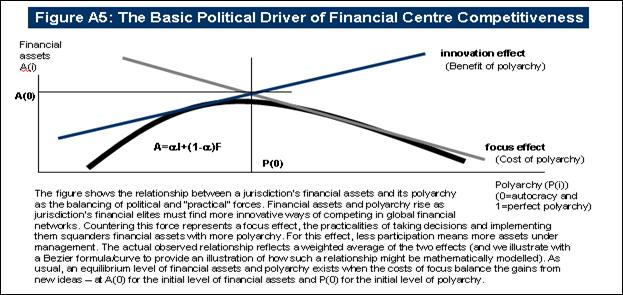
In order to figure out the effect of a foreign jurisdiction’s reactions, we first need to introduce some modifications to our model. The easiest way to do this consists of letting assets adjust according to P(j) + P*(l) where P* represents the foreign nearest jurisdiction’s level of polyarchy l such that l<j. For example, for 20 financial centres in the global network, the only jurisdiction to worry about – for the purposes of our calculation – is the one with the next highest level of polyarchy (f+f*).[149] Such a easy simplification has the simultaneous effect of reducing polyarchy levels for every level of our old polyarchy and reducing assets. Figure 6 shows the effect geometrically as a simple shift in our innovation curve. The other jurisdiction gains A(1) – A(0) assets – at our expense.[150]
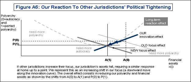
Portraying the entire network’s polyarchy,
innovation and assets thus becomes an exercise in matrix mechanics. Let A
represent a matrix of foreign assets under management (the accumulation of a
stock value) and I the matrix for the innovation stock for each country
(we do not model political capital and stability as we do not look at these in
our analysis of our research question). Namely, we don’t track how popular
governments are or preferences for stability. Let’s imagine a network of 3
countries to illustrate our model. If pim equals
the percent each i jurisdiction has attracted from jurisdiction m
in the global race of all assets under management ![]() (where pi equals the proportion of that jurisdiction’s total assets or Pi=1 for every i),
then we can portray jurisdiction’s i assets as
(where pi equals the proportion of that jurisdiction’s total assets or Pi=1 for every i),
then we can portray jurisdiction’s i assets as![]() and the whole matrix A and the corresponding
polyarchy P, as well as the amount of innovation each jurisdiction has
stored up as I. (as shown in equation (12)
and the whole matrix A and the corresponding
polyarchy P, as well as the amount of innovation each jurisdiction has
stored up as I. (as shown in equation (12)
 and
and  =
=  (12)
(12)
Modelling the interference from covariates
What effects would macroeconomic and other factors have on polyarchy and cross-borer bank liabilities? Polyarchy affects banks’ ability to attract foreign funds (through regulations) as we described above. Yet, such polyarchy naturally affects the other parts of the economy. Figure A7 shows a relatively simple model of the economy – and the way that other variables can interfere with our understanding of polyarchy’s influence on cross-border bank liabilities (and visa-versa).
Polyarchy, in the minds of most economists, probably enters the economy in the same way other political factors do – in the production function. Using the standard production function Y=aLgKg, polyarchy mainly enters through a – total factor productivity.[151] Yet, we could look at the effect such polyarchy in another way. As illustrated by Figure A8, and as already discussed in our literature review, polyarchy determines the amount of national debt, the likely propensity to invest, and even policies affect exchange rates and foreign direct investment directly. Whether polyarchy enters into these variables indirectly (by affecting upstream output) or directly (by ‘raining’ on all our variables), the result remains the same. Polyarchy has an effect on these variables in the short-run. These variables almost certainly have an endogenous effect on polyarchy in the longer-run.
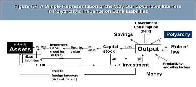

What if we could flip our perspective one more time – seeing polyarchy as the centre of the model? Figure A9 illustrates this flipped perspective, showing all these traditional variables’ effects on cross-border bank liabilities as some function of polyarchy. Because we only care about polyarchy’s effect on these assets, we can reasonably model only the effects of polyarchy on each of these variables... basically ignoring the other effects these variables have. Such a restatement allows us to express the combined effect of all these variables as one composite Q. Thus, the variable Q models all of polyarchy’s indirect effects through the various macroeconomic and other variables that affect these cross-border liabilities. As we will see the next section, such a simplification will make our econometric work much easier.

Appendix
II: Details of Econometric Procedures and Results
Fitting the macro and other factors to the data
How do we match our
model of macroeconomic and other factors into an econometric procedure? Figure
B1 shows the variables we used in our study. We divide these variables into the
groupings we use as we conduct our empirical analysis. For example, our group
of macroeconomic factors may strike as important academics who believe that
nominal prices affect the flows of these cross-border liabilities. In contrast,
financial economists might view such liabilities as the residual of any funding
not available domestically (a proposition we test with our suppliers of funds
group of variables). Thus figure thus describes these variables and what they
mean.
How can we transform these variables in
terms of the model we have already presented? In our model, cross-border assets
flow as the result of decisions about polyarchy in a jurisdiction and several
structural variables. At the end of the previous section, we explained why we
could see these variables as a composite called Q. In other words, Q=f(a,
M,F, s, K, D, d, (X-M), r, Y, w, i,e). If we take log values of the level
of these liabilities – as described in equation (6) – we get equation (13). If
we use these quantities in econometric estimation, we would obtain something
like equation (14) – where we substitute the previous beta by b in order
so we do not confuse the standard beta notation to represent regression slope
coefficients. We see that – even before worrying about the way that f transforms P
into assets, our regression coefficients would likely omit the (q-1)-1. Regression would – according to our model –
absorb all our structural parameters into the regression intercept (shown in
the bracketed term in equation (14)).
![]() (13)
(13)
![]() (14)
(14)
In practice, we did
not make these modifications for two reasons. First, we only care about the
sign of our parameter b2 – not its absolute value. Nothing in the
structural parameter q should shift in each
jurisdiction across time periods. The parameter only has the effect of scaling
our beta estimate. Second, we do not look at log values because these values do
not come out very differently from estimating levels. We thus show the values
of our variables to make reading our paper easier.
|
Figure B1: Variables Used in Our Analysis and
their Model Equivalents |
||
|
Variable |
Symbol |
Description |
|
Polyarchy (we multiplied
by 100 to make compatible with other variables) |
P |
The V-Dem’s
index of polyarchy, which measures
“the extent to which electoral democracy in its fullest sense achieved.” |
|
Cross-border
bank liabilities |
A |
Assess funds
places with a jurisdiction’s financial institutions. Liabilities in this
context refer to what we would refer to in common parlance as assets (under
management). If banks buy shares with profits, these are assets. If they take
deposits which they later repay, these are liabilities. |
|
Macroeconomic
factors – exchange rates
and interest rates both can affect the flows of funds by affecting returns
for/to foreign investors. Higher interest rates and appreciation both would
enrich foreigners, without anything in the real economy happening. |
||
|
Real exchange
rates |
e |
Exchange rates
adjusted for prices. |
|
Real interest
rates |
i |
Interest rates
adjusted for inflation and measured in percentage |
|
Attraction
factors – variables
which affect demand for foreign securities. Rising equity indices make (and
show how) these investments more valuable. GDP per capita and market
capitalisation shows the depth of equity and real markets respectively.
Deeper markets usually imply more liquidity and thus more safety. |
||
|
Market capitalization |
wK |
The amount of
money put into stock market securities, measured as a percent of GDP, and
hopefully likely a fraction of other ‘physical’ capital. |
|
GDP per
capita |
Y |
Measured in
current US dollars |
|
Stock market
value |
rK |
The value of
jurisdiction’s S&P Global Equity indices, likely in the longer run to
reflect capital’s productivity (hopefully). |
|
Connectivity
factors- these variables
gauge the extent to which one jurisdiction has contact with another. Current
account balances show how much they trade. If capital accounts must go in the
opposite direction as current accounts, then imports and exports directly
affect our model. Commercial service exports show demand for services (with
such services usually needing direct contact or at least knowledge of the foreign
market). Air transport similarly measures knowledge and even tourist demand
for a country’s currency. |
||
|
Current
account balance |
(X-M) |
Measured as a
share of GDP |
|
Commercial
service exports |
f |
in billions of
US dollars. |
|
Air transport |
d |
in millions of
passengers. |
|
Demanders of
funds – measures how
demand for funds might, independent of bank attractiveness, affect the
attractiveness of a place for these cross-border liabilities. Large
government debts require finance (some of which comes from abroad). Gross
capital formation measures real investment, the real productive motor driving
demand for such funds. |
||
|
Central
government debt |
D |
as percent of
GDP. |
|
Investment |
K |
Gross capital
formation as percent of GDP. |
|
Suppliers
of funds –
rivals for these banks providing these liabilities for later lending/use.
Savings provide more domestic financial resources, reducing the need for
foreign resources. Foreign direct investment provides funds for earmarked
projects (though these liabilities might actually represent some of these
investments). Broad money growth provides liquidity from the central bank, as
a competitor for supplier of funds. |
||
|
Savings |
sK |
Gross domestic
savings as percent of GDP. |
|
Foreign
Direct Investment |
Z |
Net flows of
such investment as percent of GDP |
|
Broad money
growth |
M |
growth expressed
in annual percentage terms. |
|
Institutional
factors – institutions
affect where investors would place their funds. Rule of law thus proxies
broader norms and laws designed to protect property rights and fair play. |
||
|
Rule of Law |
a |
An index based
on a survey of surveys. For more, see: http://databank.worldbank.org/data/databases/rule-of-law
|
Sources: Polyarchy
comes from V-Dem, cross-border bank liabilities from the Bank for International
Settlements, and all other variables come from the World Bank.
Polyarchy hardly seems to measure the extent to which multiple groups participate in political decisions – particularly the politics of specialised regulations like financial regulations. Does such a measure at least partially capture multiple groups in decision-making – particularly in much of the world where such participation occurs behind closed doors? Figure B2a shows the way we represent the variable in this study – as an intermediating case between perfect democracy and perfect autocracy. The variable contains freedom of association (which cabals and other insider groups do not rely upon). Clean elections probably reflect a broader propensity to allow for rivalry (a proxy for a very relevant propensity). Freedom of expression in public life often correlates with such freedoms in private sphere (such as in organisations). Such freedom thus probably proxies the extent to which multiple groups of insiders can express their preferences. An elected executive and suffrage more generally show s propensity for allowing very minority groups (or even one person) the chance to exercise power. Yet, these sub-components probably weight little in our overall proxy.
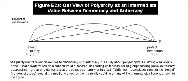
Figure B3 shows the
empirical and modeling reasons why we treat all the outside covariates as one
variable Q. In this figure, we show the correlation between polyarchies
predicted by our model and those observed in the real world. While our model
does make mistakes, we showed how these estimates do not vary much from those
obtained using machine learning techniques. These techniques treat the dataset
as one large construct – splitting it into pieces which the algorithm can
useful correlate. Thus, from an empirical view, we only need to scale polyarchy
and cross-border bank liabilities by some parameter reflecting the effect of
such Q – which we have modeled as independent of any effect of polyarchy in
equation (14).

Variables used to create network data
Which variables mattered most for building and rebuilding the international matrix of cross-border bank liabilities? In the first regression panel, we show the effect of our covariates on the extent to which cross-border bank liabilities ‘drop-off’ based on the rank a jurisdiction holds as a supplier of these liabilities. Figure B3 shows linear models analysis – a type of linear regression which takes care of problems we discussed in our paper. In this simple type of analysis, real exchange rates and interest rates fail to explain these differences – highlighting the primacy of real variables over nominal ones (a theme that remerges constantly in this study).[152] The size of the economy (broadly speaking) and the quality of its institutions have the largest predictive power on these ranks. Figure B4 tells a slightly different story. Statistically significant variables representing connectivity (in goods and people) seems to explain the lead jurisdiction placing these cross-border liabilities. Domestic investment seems to harm the prospects of attracting such funds – and savings as well (though not statistically significant). The residuals from these regressions should explain that these variables do not. We used these residuals in our study.
Figure
B3: Regression on Exponential Relationship Between Banking Liabilities of
Counterpart Jurisdictions
(statistically significant variables in bold with parameter values’ standard deviations in gray and all dependent variables adjusted to be independent of each other)*
|
Model |
Macro |
Attract |
Connect |
Demand |
Supply |
Overall* |
|
Intercept |
-0.5118 |
-0.51225 |
-0.38662 |
-0.30121 |
-0.39798 |
-0.46444 |
|
|
0.144035 |
0.019126 |
0.009638 |
0.071639 |
0.023547 |
0.011669 |
|
Real exchange rates |
0.002121 |
|
|
|
|
|
|
|
0.001415 |
|
|
|
|
|
|
Annual difference in exchange rates |
0.000003 |
|
|
|
|
|
|
|
0.00002 |
|
|
|
|
|
|
Real interest rate (%) |
-0.00177 |
|
|
|
|
|
|
|
0.001295 |
|
|
|
|
|
|
Market capitalisation |
|
0.000549 |
|
|
|
0.000496 |
|
|
|
0.000102 |
|
|
|
0.000084 |
|
GDP per capita |
|
0.003999 |
|
|
|
|
|
|
|
0.000455 |
|
|
|
|
|
Change in S&P Global Equity Indices |
-0.00024 |
|
|
|
|
|
|
|
|
0.000205 |
|
|
|
|
|
Current account balance |
0.004913 |
|
|
|
||
|
|
|
|
0.001564 |
|
|
|
|
Commercial service exports |
|
0.000815 |
|
|
0.00051 |
|
|
|
|
|
0.000096 |
|
|
0.000086 |
|
Air transport |
-0.00043 |
|
|
-0.00033 |
||
|
|
|
|
0.00008 |
|
|
0.000064 |
|
Central government debt |
|
|
0.000238 |
|
|
|
|
|
|
|
|
0.000325 |
|
|
|
Gross capital formation |
|
|
-0.00051 |
|
|
|
|
|
|
|
|
0.002624 |
|
|
|
Savings |
|
|
|
|
-0.00177 |
|
|
|
|
|
|
|
0.000891 |
|
|
Foreign Direct Investment |
|
|
|
0.003265 |
|
|
|
|
|
|
|
|
0.002023 |
|
|
Broad money growth |
|
|
|
0.000609 |
|
|
|
|
|
|
|
|
0.000938 |
|
|
Rule of Law |
|
|
|
|
0.097999 |
0.057217 |
|
|
|
|
|
|
0.007184 |
0.007254 |
The figure shows
the b-values (not beta values) for linear analysis using the variable we
described as “exponential drop off” as the dependent variable. B-values measure
the number of units (percent) change such an effect has, rather than measuring
such changes in standard deviation terms (ie as the number of standard
deviations a dependent variable reacts for a 1 standard deviation change in the
independent variable).
* Independent of
each other refers to the orthogonally we described in the main part of our
paper. We mapped our variables onto an equal number of orthogonal factors in
order to remove the high amount of correlation between all of our
variables.
Figure
B4: Regression on Lead Counterpart Jurisdiction Providing the Largest Banking
Liabilities
(statistically significant parameter values in bold with standard deviations below them in gray)
|
Model |
Mixed |
Mixed |
Mixed |
|
Intercept |
1489961 |
902856.1 |
120072.7 |
|
|
205618.2 |
118968.3 |
296585.4 |
|
Commercial service exports |
1218 |
1150.8 |
|
|
|
362.4 |
136.1 |
|
|
Savings |
-8144 |
-40994.2 |
|
|
|
8188 |
4770 |
|
|
Central government debt |
-6737 |
|
7178.3 |
|
|
2053.8 |
|
1789.6 |
|
Gross capital formation |
-42390 |
|
-36508.2 |
|
|
9249.3 |
|
9871.7 |
|
Air transport |
603 |
|
|
|
|
205.5 |
|
|
|
Rule of Law |
164512 |
177301.1 |
|
|
|
76839.9 |
30302.5 |
|
|
GDP per capita |
-5515 |
|
17473.4 |
|
|
5034.6 |
|
2339.4 |
|
Current account balance (% of GDP) |
|
19734.2 |
-29424.5 |
|
|
|
4886.1 |
5521.3 |
How much money did these lead liabilities providers and their followers-up provide in reality and according to the adjustments given by the regressions above? Figure B5a shows an example of one country, for one year. In 2005, Australia received about $35,000 in these cross-border bank liabilities from US-based natural and legal persons (people and companies). Our regression analysis though tells us the jurisdiction should have received $107,000 from the US – if we hold the relevant variables constant. Figure B5b shows lead investor for jurisdictions we analysed in this study – remembering that these jurisdictions should reflect or represent financial centres in some way. The figure only shows one value for Australia in 2005 – namely the US’s $35,000 placement in cross-border liabilities. The figure similarly ‘stacks’ all jurisdictions’ placement of funds, showing the lead placer and the drop-off coefficient as a decay coefficient. Such a figure gives the reader an idea of how much these data changed due to our ‘corrections.’ For negative values, we reversed the direction of these financial flows. Namely, if the UK, as Ireland’s pre-adjusted largest liabilities provider sent $287,000 in 2005, and should have sent -$507,000 – we simply reverse the direction of this flow for the purpose of making our network graphs.
Figure
B5a: Example of BIS original bank liabilities data before and after controlling
for outside effects
|
Reporting jurisdiction |
Counterpart country |
Amount |
New Largest |
Reporting jurisdiction |
Counterpart country |
Amount |
New Largest |
|
Australia |
US |
35110 |
106743 |
Australia |
Cayman Islands |
71 |
1262 |
|
Australia |
UK |
8588 |
79405 |
Australia |
Bermuda |
58 |
939 |
|
Australia |
Singapore |
5421 |
59069 |
Australia |
Israel |
37 |
698 |
|
Australia |
Hong Kong |
5308 |
43941 |
Australia |
South Korea |
36 |
519 |
|
Australia |
Germany |
4346 |
32687 |
Australia |
Denmark |
24 |
386 |
|
Australia |
Netherlands |
3550 |
24315 |
Australia |
Luxembourg |
23 |
287 |
|
Australia |
Japan |
3528 |
18088 |
Australia |
Jordan |
22 |
214 |
|
Australia |
New Zealand |
2085 |
13456 |
Australia |
Norway |
21 |
159 |
|
Australia |
Taiwan |
1523 |
10009 |
Australia |
UAE |
20 |
118 |
|
Australia |
China |
691 |
7446 |
Australia |
Austria |
16 |
88 |
|
Australia |
Canada |
649 |
5539 |
Australia |
Bahamas |
4 |
65 |
|
Australia |
Sweden |
189 |
4120 |
Australia |
Guernsey |
4 |
49 |
|
Australia |
Switzerland |
178 |
3065 |
Australia |
Jersey |
3 |
36 |
|
Australia |
Ireland |
146 |
2280 |
Australia |
Morocco |
1 |
27 |
|
Australia |
South Africa |
122 |
1696 |
Australia |
Qatar |
1 |
20 |
The figure shows
the value of funds in US dollars deposited by Australians in the countries
shown about for only one year (2005). We show our “corrected” amount next to
these figures, as the amount which would be deposited if not for the effect of macroeconomic
and other outside factors.
Figure
B5b: Data Used to Figure Out How Much Money Foreigners Put in Banks
|
|
|
Observed |
Predicted |
|
|
Observed |
Predicted |
||||
|
Country Name |
Year |
Largest invest (thous) |
Old decay |
New Largest Invest |
New Decays |
Country Name |
Year |
Largest invest |
Old decay |
New Largest Invest |
New Decays |
|
Australia |
2005 |
35.1 |
-0.350 |
106.7 |
-0.295 |
South Africa |
2010 |
6.68 |
-0.326 |
66.2 |
-0.331 |
|
Belgium |
2005 |
142.9 |
-0.225 |
112.3 |
-0.314 |
South Korea |
2010 |
29.3 |
-0.390 |
-215.8 |
-0.327 |
|
Brazil |
2005 |
11.8 |
-0.399 |
28.8 |
-0.454 |
Switzerland |
2010 |
159.9 |
-0.187 |
188.8 |
-0.218 |
|
France |
2005 |
316.0 |
-0.236 |
429.3 |
-0.268 |
United States |
2010 |
12,8/8.8 |
-0.284 |
1,146.8 |
-0.276 |
|
Ireland |
2005 |
289.9 |
-0.321 |
-507.6 |
-0.320 |
Australia |
2011 |
44.6 |
-0.282 |
57.8 |
-0.319 |
|
Mexico |
2005 |
1406 |
-0.617 |
-15.1 |
-0.455 |
Austria |
2011 |
56.0 |
-0.298 |
231.4 |
-0.327 |
|
Netherlands |
2005 |
182.0 |
-0.259 |
229.6 |
-0.268 |
Belgium |
2011 |
101.7 |
-0.232 |
246.4 |
-0.313 |
|
South Korea |
2005 |
13.7 |
-0.326 |
-255.3 |
-0.340 |
Brazil |
2011 |
47.5 |
-0.418 |
19.9 |
-0.456 |
|
Switzerland |
2005 |
163.9 |
-0.203 |
302.2 |
-0.197 |
Canada |
2011 |
59.5 |
-0.438 |
317.5 |
-0.291 |
|
United King. |
2005 |
635.0 |
-0.175 |
808.1 |
-0.211 |
France |
2011 |
483.6 |
-0.268 |
570.6 |
-0.253 |
|
United States |
2005 |
714.5 |
-0.260 |
748.5 |
-0.360 |
Ireland |
2011 |
177.0 |
-0.340 |
-127.2 |
-0.322 |
|
Australia |
2006 |
23.7 |
-0.295 |
74.7 |
-0.280 |
Mexico |
2011 |
11.7 |
-0.521 |
-60.3 |
-0.482 |
|
Belgium |
2006 |
136.5 |
-0.208 |
93.3 |
-0.306 |
Netherlands |
2011 |
221.8 |
-0.249 |
374.1 |
-0.268 |
|
Brazil |
2006 |
16.7 |
-0.404 |
40.3 |
-0.447 |
South Africa |
2011 |
6.0 |
-0.307 |
58.8 |
-0.362 |
|
France |
2006 |
483.1 |
-0.243 |
438.3 |
-0.251 |
South Korea |
2011 |
33.5 |
-0.397 |
-199.4 |
-0.335 |
|
Ireland |
2006 |
406.8 |
-0.341 |
-419.9 |
-0.304 |
Switzerland |
2011 |
149.7 |
-0.188 |
50.7 |
-0.241 |
|
Mexico |
2006 |
3.6 |
-0.580 |
-83.0 |
-0.458 |
United States |
2011 |
116.34 |
-0.266 |
1,223.6 |
-0.257 |
|
Netherlands |
2006 |
232.5 |
-0.274 |
246.0 |
-0.257 |
Australia |
2012 |
5.57 |
-0.284 |
37.0 |
-0.320 |
|
South Korea |
2006 |
30.8 |
-0.353 |
-244.1 |
-0.346 |
Austria |
2012 |
5.85 |
-0.324 |
237.0 |
-0.326 |
|
Switzerland |
2006 |
148.9 |
-0.182 |
215.1 |
-0.177 |
Belgium |
2012 |
7.32 |
-0.205 |
298.5 |
-0.307 |
|
UK |
2006 |
780.2 |
-0.175 |
842.9 |
-0.176 |
Brazil |
2012 |
4.25 |
-0.403 |
52.0 |
-0.461 |
|
United States |
2006 |
990.4 |
-0.270 |
801.6 |
-0.334 |
Canada |
2012 |
23.41 |
-0.463 |
304.3 |
-0.292 |
|
Australia |
2007 |
34.7 |
-0.286 |
37.1 |
-0.277 |
France |
2012 |
42.96 |
-0.251 |
565.1 |
-0.252 |
|
Austria |
2007 |
55.2 |
-0.250 |
208.2 |
-0.289 |
Ireland |
2012 |
11.28 |
-0.336 |
-106.4 |
-0.323 |
|
Belgium |
2007 |
200.24 |
-0.217 |
92.0 |
-0.303 |
Mexico |
2012 |
.79 |
-0.498 |
-100.6 |
-0.480 |
|
Brazil |
2007 |
2.3 |
-0.373 |
-3.0 |
-0.432 |
Netherlands |
2012 |
22.42 |
-0.260 |
418.7 |
-0.266 |
Figure
B5b Continued
|
Country Name |
Year |
Largest invest (thous) |
Old decay |
New Largest Invest |
New Decays |
Country Name |
Year |
Largest invest |
Old decay |
New Largest Invest |
New Decays |
|
Canada |
2007 |
6.0 |
-0.375 |
250.2 |
-0.261 |
South Africa |
2012 |
.77 |
-0.326 |
82.1 |
-0.346 |
|
France |
2007 |
65.9 |
-0.240 |
447.2 |
-0.239 |
South Korea |
2012 |
1.15 |
-0.311 |
-108.3 |
-0.325 |
|
Ireland |
2007 |
50.1 |
-0.327 |
-332.0 |
-0.309 |
Switzerland |
2012 |
11.50 |
-0.176 |
133.3 |
-0.227 |
|
Mexico |
2007 |
.3 |
-0.546 |
-86.3 |
-0.463 |
United States |
2012 |
10.061 |
-0.258 |
1,216.1 |
-0.239 |
|
Netherlands |
2007 |
33.4 |
-0.277 |
199.3 |
-0.246 |
Australia |
2013 |
.465 |
-0.271 |
98.5 |
-0.324 |
|
South Korea |
2007 |
3.4 |
-0.338 |
-195.1 |
-0.324 |
Austria |
2013 |
.648 |
-0.328 |
260.3 |
-0.325 |
|
Switzerland |
2007 |
32.0 |
-0.206 |
75.0 |
-0.179 |
Belgium |
2013 |
.692 |
-0.206 |
323.6 |
-0.299 |
|
United King. |
2007 |
97.64 |
-0.173 |
869.5 |
-0.165 |
Brazil |
2013 |
.302 |
-0.467 |
75.9 |
-0.470 |
|
United States |
2007 |
11.4 |
-0.274 |
918.6 |
-0.306 |
Canada |
2013 |
2.245 |
-0.448 |
296.8 |
-0.294 |
|
Australia |
2008 |
.27 |
-0.304 |
81.4 |
-0.321 |
France |
2013 |
4.139 |
-0.246 |
592.6 |
-0.238 |
|
Austria |
2008 |
.59 |
-0.284 |
227.4 |
-0.311 |
Ireland |
2013 |
1.228 |
-0.382 |
-67.4 |
-0.309 |
|
Belgium |
2008 |
1.57 |
-0.230 |
159.5 |
-0.318 |
Mexico |
2013 |
.133 |
-0.525 |
-70.8 |
-0.483 |
|
Brazil |
2008 |
.22 |
-0.391 |
-31.1 |
-0.464 |
Netherlands |
2013 |
1.544 |
-0.258 |
400.9 |
-0.257 |
|
Canada |
2008 |
.67 |
-0.426 |
252.6 |
-0.303 |
South Africa |
2013. |
52 |
-0.298 |
59.9 |
-0.332 |
|
France |
2008 |
5.32 |
-0.243 |
492.1 |
-0.251 |
South Korea |
2013. |
55 |
-0.296 |
-84.5 |
-0.336 |
|
Ireland |
2008 |
4.16 |
-0.322 |
-162.1 |
-0.330 |
Switzerland |
2013 |
1.058 |
-0.180 |
156.7 |
-0.208 |
|
Mexico |
2008. |
92 |
-0.539 |
-140.2 |
-0.483 |
United States |
2013 |
1.1890 |
-0.253 |
1,227.2 |
-0.210 |
|
Netherlands |
2008 |
2.62 |
-0.266 |
182.2 |
-0.277 |
Australia |
2014. |
987 |
-0.283 |
143.5 |
-0.318 |
|
South Korea |
2008 |
.38 |
-0.356 |
-184.0 |
-0.350 |
Austria |
2014. |
727 |
-0.322 |
266.4 |
-0.323 |
|
Switzerland |
2008 |
1.62 |
-0.189 |
-92.7 |
-0.232 |
Belgium |
2014. |
717 |
-0.196 |
316.5 |
-0.291 |
|
United King. |
2008 |
8.66 |
-0.183 |
894.7 |
-0.205 |
Brazil |
2014. |
439 |
-0.440 |
121.9 |
-0.474 |
|
United States |
2008 |
1.22 |
-0.266 |
1041.4 |
-0.298 |
Canada |
2014. |
961 |
-0.357 |
322.2 |
-0.290 |
|
Australia |
2009. |
337 |
-0.302 |
4.8 |
-0.292 |
France |
2014 |
.3164 |
-0.239 |
619.1 |
-0.232 |
|
Austria |
2009. |
497 |
-0.258 |
272.9 |
-0.321 |
Ireland |
2014. |
116 |
-0.378 |
-194.2 |
-0.310 |
|
Belgium |
2009 |
.1541 |
-0.231 |
250.0 |
-0.310 |
Switzerland |
2014. |
760 |
-0.176 |
136.8 |
-0.203 |
|
Brazil |
2009. |
611 |
-0.366 |
122.5 |
-0.440 |
United States |
2014 |
.15747 |
-0.243 |
1,275.3 |
-0.190 |
|
Canada |
2009. |
422 |
-0.426 |
399.7 |
-0.281 |
Australia |
201.5 |
7952 |
-0.284 |
160.1 |
-0.329 |
|
France |
2009 |
.4695 |
-0.255 |
551.1 |
-0.261 |
Austria |
201.5 |
1664 |
-0.303 |
208.0 |
-0.334 |
|
Ireland |
2009 |
.4559 |
-0.359 |
-117.1 |
-0.332 |
Belgium |
201.5 |
5323 |
-0.195 |
279.2 |
-0.294 |
|
Mexico |
200.9 |
775 |
-0.541 |
-77.1 |
-0.471 |
Brazil |
201.5 |
9577 |
-0.432 |
176.0 |
-0.490 |
|
Netherlands |
2009 |
.2622 |
-0.278 |
325.9 |
-0.269 |
Canada |
201.5 |
0219 |
-0.341 |
373.8 |
-0.308 |
|
South Africa |
200.9 |
724 |
-0.350 |
21.4 |
-0.318 |
France |
2015. |
4590 |
-0.239 |
571.3 |
-0.250 |
|
South Korea |
2009. |
748 |
-0.391 |
-124.0 |
-0.333 |
Ireland |
201.5 |
6902 |
-0.375 |
-615.5 |
-0.323 |
|
Switzerland |
2009 |
.1624 |
-0.189 |
76.7 |
-0.222 |
Mexico |
20.15 |
8023 |
-0.506 |
-66.3 |
-0.489 |
|
United States |
2009 |
.11732 |
-0.284 |
1094.5 |
-0.294 |
Netherlands |
2015. |
8269 |
-0.294 |
355.2 |
-0.255 |
|
Australia |
201.0 |
5281 |
-0.285 |
101.4 |
-0.298 |
South Africa |
20.15 |
9415 |
-0.314 |
44.7 |
-0.356 |
|
Austria |
201.0 |
8197 |
-0.302 |
275.2 |
-0.323 |
South Korea |
201.5 |
2688 |
-0.313 |
-140.2 |
-0.352 |
|
Belgium |
2010. |
1507 |
-0.231 |
289.7 |
-0.309 |
Spain |
201.5 |
5952 |
-0.328 |
302.8 |
-0.352 |
|
Brazil |
201.0 |
8688 |
-0.399 |
25.6 |
-0.437 |
Switzerland |
2015. |
4465 |
-0.209 |
178.5 |
-0.206 |
|
Canada |
2010. |
7363 |
-0.467 |
352.2 |
-0.277 |
United States |
2015. |
7189 |
-0.236 |
1,260.4 |
-0.208 |
|
France |
2010. |
3516 |
-0.246 |
565.7 |
-0.257 |
|
|
|
|
|
|
|
Ireland |
2010. |
7796 |
-0.353 |
-53.4 |
-0.333 |
|
|
|
|
|
|
|
Mexico |
201.0 |
0842 |
-0.598 |
-42.0 |
-0.476 |
|
|
|
|
|
|
|
Netherlands |
2010. |
4009 |
-0.272 |
333.9 |
-0.266 |
|
|
|
|
. |
.......................... |
Matrix Statistics for Banking Liability Data
Jurisdictions often changed their network position radically as a result of these adjustments. Figure B6 shows the pre-adjustment average eigencentrality, cluster centrality, Pagerank, authority and hub values for the jurisdictions we studied. Figure B7 shows these values after our adjustments on a year-by-year basis. In this way, interested readers can see – or use – these data.
Figure
B6: Multiple Matrix Statistics Before Adjustment
|
Eigenvalue centrality |
|
cluster
centrality |
|
Pagerank
average |
|
Authority |
|
Hub |
|||||
|
Germany |
99.97 |
|
Jordan |
86.26 |
|
UK |
3.83 |
|
Germany |
19.76 |
|
Ireland |
56.75 |
|
Japan |
99.51 |
|
Qatar |
84.23 |
|
US |
3.73 |
|
Japan |
19.53 |
|
US |
55.69 |
|
Singapore |
98.89 |
|
Bermuda |
80.24 |
|
Germany |
3.61 |
|
Singapore |
19.36 |
|
Isle of Man |
55.16 |
|
Hong Kong |
98.39 |
|
New Zealand |
79.76 |
|
Canada |
3.37 |
|
Canada |
19.34 |
|
Guernsey |
53.68 |
|
Norway |
96.04 |
|
UAE |
73.57 |
|
Switzerland |
3.36 |
|
Hong Kong |
19.22 |
|
Brazil |
53.05 |
|
Bermuda |
95.87 |
|
Israel |
72.99 |
|
France |
3.32 |
|
Norway |
19.03 |
|
Finland |
52.28 |
|
Canada |
95.00 |
|
Morocco |
71.21 |
|
Netherlands |
3.24 |
|
Netherlands |
18.98 |
|
Chile |
50.81 |
|
China |
94.56 |
|
Bahamas |
70.25 |
|
Japan |
3.23 |
|
UK |
18.80 |
|
Mexico |
50.71 |
|
Netherlands |
94.05 |
|
Norway |
68.55 |
|
Singapore |
3.16 |
|
Switzerland |
18.64 |
|
Canada |
48.82 |
|
UK |
93.62 |
|
Singapore |
68.15 |
|
Ireland |
3.14 |
|
France |
18.55 |
|
Belgium |
48.50 |
|
Ireland |
93.61 |
|
Cayman Islands |
67.81 |
|
Hong Kong |
3.13 |
|
US |
18.54 |
|
Jersey |
47.92 |
|
Switzerland |
93.61 |
|
China |
66.97 |
|
Luxembourg |
3.05 |
|
China |
18.41 |
|
Luxembourg |
47.81 |
|
US |
93.59 |
|
Germany |
66.16 |
|
Cayman Islands |
2.98 |
|
Sweden |
18.37 |
|
Switzerland |
47.80 |
|
Luxembourg |
93.08 |
|
Hong Kong |
65.54 |
|
China |
2.87 |
|
Cayman Islands |
18.26 |
|
France |
47.80 |
|
Australia |
92.60 |
|
Japan |
63.30 |
|
Sweden |
2.81 |
|
Ireland |
18.24 |
|
UK |
47.79 |
|
France |
91.98 |
|
Mexico |
60.38 |
|
Australia |
2.70 |
|
Luxembourg |
18.21 |
|
Denmark |
47.20 |
|
Austria |
91.16 |
|
South Africa |
58.86 |
|
Bahamas |
2.57 |
|
Austria |
18.17 |
|
Sweden |
47.02 |
|
South Africa |
90.79 |
|
Greece |
58.79 |
|
Norway |
2.53 |
|
Denmark |
17.94 |
|
Netherlands |
46.25 |
|
Israel |
90.43 |
|
Netherlands |
56.12 |
|
Bermuda |
2.52 |
|
Australia |
17.82 |
|
Austria |
45.03 |
|
Cayman Islands |
90.29 |
|
Isle of Man |
53.36 |
|
Austria |
2.49 |
|
South Africa |
17.71 |
|
South Africa |
40.24 |
|
Denmark |
89.88 |
|
Finland |
53.20 |
|
Denmark |
2.48 |
|
Bahamas |
17.21 |
|
Greece |
39.56 |
|
Sweden |
89.42 |
|
Guernsey |
52.96 |
|
Jersey |
2.48 |
|
Taiwan |
17.19 |
|
Taiwan |
38.58 |
|
UAE |
88.25 |
|
Brazil |
52.58 |
|
UAE |
2.41 |
|
Israel |
17.18 |
|
Australia |
38.53 |
|
Taiwan |
88.05 |
|
Chile |
51.91 |
|
Taiwan |
2.40 |
|
South Korea |
17.18 |
|
South Korea |
36.62 |
|
New Zealand |
88.00 |
|
Canada |
51.13 |
|
South Africa |
2.37 |
|
Bermuda |
17.11 |
|
Bahamas |
36.36 |
|
South Korea |
87.91 |
|
Austria |
49.77 |
|
South Korea |
2.30 |
|
UAE |
16.82 |
|
Cayman Islands |
36.36 |
|
Bahamas |
86.31 |
|
Belgium |
47.98 |
|
Israel |
2.29 |
|
New Zealand |
16.08 |
|
Germany |
36.36 |
|
Jersey |
85.10 |
|
South Korea |
47.06 |
|
Guernsey |
2.27 |
|
Jersey |
15.36 |
|
Japan |
36.36 |
|
Jordan |
79.21 |
|
Jersey |
46.03 |
|
New Zealand |
2.07 |
|
Guernsey |
14.67 |
|
Morocco |
33.89 |
|
Guernsey |
77.71 |
|
US |
45.27 |
|
Jordan |
1.93 |
|
Morocco |
13.82 |
|
Bermuda |
27.27 |
|
Morocco |
74.59 |
|
Taiwan |
44.61 |
|
Qatar |
1.92 |
|
Jordan |
13.81 |
|
Israel |
27.27 |
|
Qatar |
73.21 |
|
Denmark |
44.44 |
|
Morocco |
1.81 |
|
Qatar |
13.07 |
|
Jordan |
27.27 |
|
Belgium |
0.00 |
|
Australia |
44.29 |
|
Belgium |
1.26 |
|
Belgium |
0.00 |
|
New Zealand |
27.27 |
|
Brazil |
0.00 |
|
Luxembourg |
43.51 |
|
Brazil |
1.26 |
|
Brazil |
0.00 |
|
Norway |
27.27 |
|
Chile |
0.00 |
|
Switzerland |
43.01 |
|
Chile |
1.26 |
|
Chile |
0.00 |
|
Qatar |
27.27 |
|
Finland |
0.00 |
|
France |
42.82 |
|
Finland |
1.26 |
|
Finland |
0.00 |
|
UAE |
27.27 |
|
Greece |
0.00 |
|
UK |
42.72 |
|
Greece |
1.26 |
|
Greece |
0.00 |
|
Hong Kong |
21.94 |
|
Isle of Man |
0.00 |
|
Ireland |
42.36 |
|
Isle of Man |
1.26 |
|
Isle of Man |
0.00 |
|
China |
18.18 |
|
Macao |
0.00 |
|
Sweden |
42.27 |
|
Macao |
1.26 |
|
Macao |
0.00 |
|
Singapore |
18.18 |
|
Mexico |
0.00 |
|
Macao |
14.97 |
|
Mexico |
1.26 |
|
Mexico |
0.00 |
|
Spain |
12.98 |
|
Spain |
0.00 |
|
Spain |
9.75 |
|
Spain |
1.26 |
|
Spain |
0.00 |
|
Macao |
5.64 |
Figure
B7: Multiple Matrix Statistics After Adjustment
|
Country |
Year |
authority |
hub |
page-ranks |
cluster-ing |
eigen- |
authority |
year |
authoity |
hub |
page- cluster rank |
eigen |
|
|
Australia |
2005 |
0.164 |
0.354 |
0.005 |
0.223 |
0.134 |
South
Korea |
2010 |
0.234 |
0.025 |
0.245 |
0.310 |
0.889 |
|
Belgium |
2005 |
|
0.375 |
0.005 |
0.220 |
|
Sweden |
2010 |
0.178 |
0.040 |
0.010 |
0.591 |
0.178 |
|
Brazil |
2005 |
|
0.284 |
0.005 |
0.316 |
|
Switzerland |
2010 |
0.169 |
0.361 |
0.011 |
0.238 |
0.178 |
|
Canada |
2005 |
0.188 |
0.040 |
0.006 |
0.582 |
0.161 |
United
Kingdom |
2010 |
0.193 |
0.040 |
0.012 |
0.614 |
0.208 |
|
China |
2005 |
0.188 |
0.040 |
0.006 |
0.582 |
0.161 |
United
States |
2010 |
0.171 |
0.336 |
0.012 |
0.268 |
0.178 |
|
Denmark |
2005 |
0.188 |
0.031 |
0.006 |
0.656 |
0.161 |
Australia |
2011 |
0.169 |
0.353 |
0.010 |
0.251 |
0.175 |
|
Finland |
2005 |
|
|
0.005 |
|
|
Austria |
2011 |
0.178 |
0.043 |
0.010 |
0.600 |
0.175 |
|
France |
2005 |
0.139 |
0.374 |
0.006 |
0.218 |
0.111 |
Belgium |
2011 |
0.000 |
0.361 |
0.008 |
0.235 |
0.000 |
|
Germany |
2005 |
0.188 |
0.040 |
0.006 |
0.582 |
0.161 |
Brazil |
2011 |
0.000 |
0.291 |
0.008 |
0.332 |
0.000 |
|
Greece |
2005 |
|
|
0.005 |
|
|
Canada |
2011 |
0.178 |
0.220 |
0.011 |
0.385 |
0.175 |
|
Hungary |
2005 |
|
|
|
|
|
Denmark |
2011 |
0.178 |
0.043 |
0.010 |
0.600 |
0.175 |
|
Ireland |
2005 |
0.236 |
0.016 |
0.396 |
0.237 |
1.000 |
Finland |
2011 |
0.000 |
0.000 |
0.008 |
0.000 |
0.000 |
|
Israel |
2005 |
0.148 |
0.031 |
0.005 |
0.679 |
0.132 |
France |
2011 |
0.154 |
0.362 |
0.011 |
0.242 |
0.149 |
|
Mexico |
2005 |
0.133 |
|
0.012 |
0.500 |
0.290 |
Ireland |
2011 |
0.245 |
0.016 |
0.192 |
0.251 |
1.000 |
|
Morocco |
2005 |
0.148 |
0.016 |
0.005 |
0.714 |
0.132 |
Mexico |
2011 |
0.167 |
0.000 |
0.170 |
0.293 |
0.762 |
|
Netherlands |
2005 |
0.167 |
0.316 |
0.006 |
0.275 |
0.134 |
Netherlands |
2011 |
0.172 |
0.310 |
0.011 |
0.307 |
0.175 |
|
South
Korea |
2005 |
0.230 |
0.016 |
0.381 |
0.289 |
0.885 |
Qatar |
2011 |
0.094 |
0.032 |
0.009 |
0.633 |
0.087 |
|
Sweden |
2005 |
0.188 |
0.040 |
0.006 |
0.582 |
0.161 |
Singapore |
2011 |
0.192 |
0.043 |
0.011 |
0.614 |
0.204 |
|
Switzerland |
2005 |
0.163 |
0.373 |
0.006 |
0.217 |
0.134 |
South
Africa |
2011 |
0.156 |
0.334 |
0.009 |
0.257 |
0.149 |
|
United
Kingdom |
2005 |
0.163 |
0.373 |
0.006 |
0.217 |
0.134 |
South
Korea |
2011 |
0.238 |
0.027 |
0.252 |
0.297 |
0.910 |
|
United
States |
2005 |
0.165 |
0.336 |
0.006 |
0.255 |
0.134 |
Sweden |
2011 |
0.178 |
0.043 |
0.010 |
0.600 |
0.175 |
|
Australia |
2006 |
0.143 |
0.363 |
0.005 |
0.228 |
0.133 |
Switzerland |
2011 |
0.169 |
0.361 |
0.011 |
0.241 |
0.175 |
|
Belgium |
2006 |
0.000 |
0.370 |
0.005 |
0.223 |
0.000 |
United
Kingdom |
2011 |
0.192 |
0.043 |
0.012 |
0.614 |
0.204 |
|
Brazil |
2006 |
0.000 |
0.271 |
0.005 |
0.290 |
0.000 |
United
States |
2011 |
0.170 |
0.337 |
0.012 |
0.270 |
0.175 |
|
Denmark |
2006 |
0.168 |
0.044 |
0.006 |
0.644 |
0.159 |
Australia |
2012 |
0.147 |
0.355 |
0.011 |
0.244 |
0.167 |
|
Finland |
2006 |
0.000 |
0.000 |
0.005 |
0.000 |
0.000 |
Austria |
2012 |
0.172 |
0.044 |
0.011 |
0.609 |
0.168 |
|
France |
2006 |
0.161 |
0.370 |
0.006 |
0.225 |
0.134 |
Belgium |
2012 |
0.000 |
0.352 |
0.009 |
0.241 |
0.000 |
|
Ireland |
2006 |
0.241 |
0.016 |
0.391 |
0.228 |
1.000 |
Brazil |
2012 |
0.000 |
0.293 |
0.009 |
0.282 |
0.000 |
|
Mexico |
2006 |
0.172 |
0.000 |
0.020 |
0.375 |
0.465 |
Canada |
2012 |
0.172 |
0.251 |
0.012 |
0.371 |
0.168 |
|
Netherlands |
2006 |
0.165 |
0.315 |
0.006 |
0.284 |
0.134 |
Denmark |
2012 |
0.189 |
0.044 |
0.011 |
0.629 |
0.196 |
|
South
Korea |
2006 |
0.236 |
0.016 |
0.376 |
0.279 |
0.895 |
Finland |
2012 |
0.000 |
0.000 |
0.009 |
0.000 |
0.000 |
|
Sweden |
2006 |
0.186 |
0.044 |
0.006 |
0.591 |
0.160 |
France |
2012 |
0.166 |
0.354 |
0.012 |
0.251 |
0.168 |
|
Switzerland |
2006 |
0.161 |
0.370 |
0.006 |
0.225 |
0.134 |
Ireland |
2012 |
0.247 |
0.028 |
0.183 |
0.256 |
0.991 |
|
United
Kingdom |
2006 |
0.161 |
0.370 |
0.006 |
0.225 |
0.134 |
Mexico |
2012 |
0.197 |
0.000 |
0.203 |
0.308 |
1.000 |
|
United
States |
2006 |
0.163 |
0.343 |
0.006 |
0.252 |
0.134 |
Netherlands |
2012 |
0.169 |
0.301 |
0.012 |
0.316 |
0.168 |
|
Australia |
2007 |
0.157 |
0.369 |
0.011 |
0.241 |
0.171 |
South
Africa |
2012 |
0.152 |
0.322 |
0.010 |
0.297 |
0.144 |
|
Austria |
2007 |
0.163 |
0.057 |
0.011 |
0.609 |
0.171 |
South
Korea |
2012 |
0.241 |
0.029 |
0.190 |
0.298 |
0.908 |
|
Belgium |
2007 |
0.000 |
0.353 |
0.009 |
0.243 |
0.000 |
Sweden |
2012 |
0.172 |
0.044 |
0.011 |
0.609 |
0.168 |
|
Brazil |
2007 |
0.201 |
0.000 |
0.096 |
0.379 |
0.845 |
Switzerland |
2012 |
0.166 |
0.354 |
0.012 |
0.251 |
0.168 |
|
Canada |
2007 |
0.163 |
0.278 |
0.011 |
0.330 |
0.171 |
United
Kingdom |
2012 |
0.189 |
0.044 |
0.013 |
0.629 |
0.196 |
|
Denmark |
2007 |
0.163 |
0.043 |
0.011 |
0.656 |
0.171 |
United
States |
2012 |
0.166 |
0.344 |
0.013 |
0.259 |
0.168 |
|
Finland |
2007 |
0.000 |
0.000 |
0.009 |
0.000 |
0.000 |
Australia |
2013 |
0.180 |
0.219 |
0.028 |
0.453 |
0.939 |
|
France |
2007 |
0.157 |
0.369 |
0.012 |
0.241 |
0.171 |
Austria |
2013 |
0.182 |
0.206 |
0.025 |
0.447 |
0.882 |
|
Ireland |
2007 |
0.241 |
0.028 |
0.185 |
0.246 |
1.000 |
Belgium |
2013 |
0.000 |
0.227 |
0.012 |
0.495 |
0.000 |
|
Mexico |
2007 |
0.188 |
0.000 |
0.114 |
0.458 |
0.575 |
Brazil |
2013 |
0.000 |
0.169 |
0.012 |
0.547 |
0.000 |
|
Netherlands |
2007 |
0.160 |
0.312 |
0.012 |
0.302 |
0.171 |
Canada |
2013 |
0.191 |
0.140 |
0.034 |
0.513 |
0.940 |
|
South
Korea |
2007 |
0.233 |
0.041 |
0.194 |
0.308 |
0.857 |
Denmark |
2013 |
0.166 |
0.208 |
0.024 |
0.482 |
0.828 |
|
Sweden |
2007 |
0.163 |
0.044 |
0.011 |
0.667 |
0.171 |
Finland |
2013 |
0.000 |
0.159 |
0.012 |
0.541 |
0.000 |
|
Switzerland |
2007 |
0.157 |
0.369 |
0.012 |
0.241 |
0.171 |
France |
2013 |
0.180 |
0.219 |
0.033 |
0.454 |
0.939 |
|
United
Kingdom |
2007 |
0.157 |
0.369 |
0.012 |
0.241 |
0.171 |
Ireland |
2013 |
0.181 |
0.219 |
0.031 |
0.432 |
0.939 |
|
United
States |
2007 |
0.158 |
0.341 |
0.012 |
0.269 |
0.171 |
Mexico |
2013 |
0.000 |
0.197 |
0.012 |
0.561 |
0.000 |
|
Australia |
2008 |
0.146 |
0.363 |
0.011 |
0.237 |
0.119 |
Netherlands |
2013 |
0.188 |
0.181 |
0.032 |
0.526 |
0.939 |
|
Austria |
2008 |
0.154 |
0.076 |
0.011 |
0.622 |
0.119 |
South
Africa |
2013 |
0.187 |
0.201 |
0.025 |
0.485 |
0.939 |
|
Belgium |
2008 |
0.000 |
0.366 |
0.009 |
0.233 |
0.000 |
South
Korea |
2013 |
0.174 |
0.220 |
0.024 |
0.455 |
0.892 |
|
Brazil |
2008 |
0.219 |
0.000 |
0.135 |
0.294 |
0.982 |
Sweden |
2013 |
0.183 |
0.213 |
0.028 |
0.435 |
0.883 |
|
Canada |
2008 |
0.154 |
0.248 |
0.011 |
0.405 |
0.119 |
Switzerland |
2013 |
0.187 |
0.219 |
0.034 |
0.445 |
0.939 |
|
China |
2008 |
0.172 |
0.076 |
0.011 |
0.645 |
0.143 |
United
Kingdom |
2013 |
0.187 |
0.219 |
0.039 |
0.445 |
0.939 |
|
Denmark |
2008 |
0.154 |
0.090 |
0.011 |
0.573 |
0.119 |
United
States |
2013 |
0.181 |
0.213 |
0.038 |
0.455 |
0.939 |
|
Finland |
2008 |
0.000 |
0.000 |
0.009 |
0.000 |
0.000 |
Australia |
2014 |
0.160 |
0.323 |
|
0.266 |
0.284 |
|
France |
2008 |
0.145 |
0.386 |
0.011 |
0.234 |
0.119 |
Austria |
2014 |
0.191 |
0.010 |
|
0.712 |
0.364 |
|
Ireland |
2008 |
0.294 |
0.069 |
0.138 |
0.236 |
1.000 |
Belgium |
2014 |
0.000 |
0.322 |
|
0.260 |
0.000 |
|
Mexico |
2008 |
0.200 |
0.000 |
0.083 |
0.462 |
0.662 |
Brazil |
2014 |
0.000 |
0.267 |
|
0.323 |
0.000 |
|
Netherlands |
2008 |
0.148 |
0.334 |
0.011 |
0.295 |
0.119 |
Canada |
2014 |
0.175 |
0.276 |
|
0.303 |
0.322 |
|
South
Korea |
2008 |
0.275 |
0.057 |
0.112 |
0.302 |
0.899 |
Denmark |
2014 |
0.191 |
0.010 |
|
0.712 |
0.364 |
|
Sweden |
2008 |
0.154 |
0.090 |
0.011 |
0.573 |
0.119 |
Finland |
2014 |
0.000 |
0.000 |
|
0.000 |
0.000 |
|
Switzerland |
2008 |
0.294 |
0.069 |
0.138 |
0.236 |
1.000 |
France |
2014 |
0.160 |
0.323 |
|
0.266 |
0.284 |
|
United
Kingdom |
2008 |
0.145 |
0.386 |
0.011 |
0.234 |
0.119 |
Ireland |
2014 |
0.172 |
0.322 |
|
0.265 |
0.322 |
|
United
States |
2008 |
0.146 |
0.362 |
0.011 |
0.262 |
0.119 |
Mexico |
2014 |
0.164 |
0.000 |
|
0.368 |
1.000 |
|
Australia |
2009 |
0.149 |
0.355 |
0.010 |
0.241 |
0.176 |
Netherlands |
2014 |
0.179 |
0.205 |
|
0.349 |
0.322 |
|
Austria |
2009 |
0.177 |
0.042 |
0.009 |
0.591 |
0.177 |
South
Africa |
2014 |
0.146 |
0.296 |
|
0.296 |
0.245 |
|
Belgium |
2009 |
0.000 |
0.361 |
0.008 |
0.236 |
0.000 |
South
Korea |
2014 |
0.160 |
0.323 |
|
0.266 |
0.284 |
|
Brazil |
2009 |
0.000 |
0.301 |
0.008 |
0.280 |
0.000 |
Spain |
2014 |
0.000 |
0.000 |
|
0.000 |
0.000 |
|
Canada |
2009 |
0.177 |
0.230 |
0.010 |
0.383 |
0.177 |
Sweden |
2014 |
0.175 |
0.010 |
|
0.773 |
0.363 |
|
Denmark |
2009 |
0.177 |
0.042 |
0.009 |
0.591 |
0.177 |
Switzerland |
2014 |
0.172 |
0.322 |
|
0.265 |
0.322 |
|
Finland |
2009 |
0.000 |
0.000 |
0.008 |
0.000 |
0.000 |
United
Kingdom |
2014 |
0.191 |
0.010 |
|
0.712 |
0.364 |
|
France |
2009 |
0.169 |
0.360 |
0.011 |
0.239 |
0.177 |
United
States |
2014 |
0.173 |
0.314 |
|
0.275 |
0.322 |
|
Ireland |
2009 |
0.242 |
0.026 |
0.280 |
0.253 |
1.000 |
Australia |
2015 |
0.130 |
0.355 |
0.010 |
0.252 |
0.135 |
|
Mexico |
2009 |
0.157 |
0.000 |
0.146 |
0.371 |
0.653 |
Austria |
2015 |
0.187 |
0.044 |
0.011 |
0.614 |
0.187 |
|
Netherlands |
2009 |
0.172 |
0.308 |
0.010 |
0.302 |
0.177 |
Belgium |
2015 |
0.000 |
0.351 |
0.009 |
0.249 |
0.000 |
|
South
Africa |
2009 |
0.156 |
0.327 |
0.009 |
0.270 |
0.152 |
Brazil |
2015 |
0.000 |
0.265 |
0.009 |
0.267 |
0.000 |
|
South
Korea |
2009 |
0.239 |
0.016 |
0.216 |
0.286 |
0.935 |
Canada |
2015 |
0.168 |
0.305 |
0.011 |
0.291 |
0.159 |
|
Sweden |
2009 |
0.177 |
0.042 |
0.009 |
0.591 |
0.177 |
Denmark |
2015 |
0.170 |
0.044 |
0.010 |
0.673 |
0.185 |
|
Switzerland |
2009 |
0.169 |
0.360 |
0.010 |
0.239 |
0.177 |
Finland |
2015 |
0.000 |
0.000 |
0.009 |
0.000 |
0.000 |
|
United
Kingdom |
2009 |
0.193 |
0.042 |
0.011 |
0.614 |
0.207 |
France |
2015 |
0.165 |
0.353 |
0.012 |
0.256 |
0.159 |
|
United
States |
2009 |
0.171 |
0.335 |
0.011 |
0.269 |
0.177 |
Germany |
2015 |
0.187 |
0.044 |
0.012 |
0.614 |
0.187 |
|
Australia |
2010 |
0.170 |
0.352 |
0.011 |
0.238 |
0.178 |
Ireland |
2015 |
0.249 |
0.029 |
0.191 |
0.260 |
1.000 |
|
Austria |
2010 |
0.178 |
0.040 |
0.010 |
0.591 |
0.178 |
Mexico |
2015 |
0.197 |
0.000 |
0.190 |
0.323 |
0.974 |
|
Belgium |
2010 |
0.000 |
0.363 |
0.008 |
0.235 |
0.000 |
Netherlands |
2015 |
0.170 |
0.268 |
0.011 |
0.342 |
0.159 |
|
Brazil |
2010 |
0.000 |
0.302 |
0.008 |
0.318 |
0.000 |
South
Africa |
2015 |
0.149 |
0.328 |
0.010 |
0.282 |
0.158 |
|
Canada |
2010 |
0.178 |
0.230 |
0.011 |
0.383 |
0.178 |
South
Korea |
2015 |
0.249 |
0.029 |
0.212 |
0.260 |
1.000 |
|
Denmark |
2010 |
0.178 |
0.040 |
0.010 |
0.591 |
0.178 |
Spain |
2015 |
0.000 |
0.000 |
0.009 |
0.000 |
0.000 |
|
Finland |
2010 |
0.000 |
0.000 |
0.008 |
0.000 |
0.000 |
Sweden |
2015 |
0.168 |
0.044 |
0.011 |
0.591 |
0.159 |
|
France |
2010 |
0.169 |
0.361 |
0.012 |
0.238 |
0.178 |
Switzerland |
2015 |
0.165 |
0.353 |
0.011 |
0.256 |
0.159 |
|
Ireland |
2010 |
0.240 |
0.015 |
0.181 |
0.253 |
1.000 |
United
Kingdom |
2015 |
0.187 |
0.044 |
0.013 |
0.614 |
0.187 |
|
Mexico |
2010 |
0.134 |
0.000 |
0.178 |
0.313 |
0.639 |
United
States |
2015 |
0.145 |
0.345 |
0.012 |
0.266 |
0.136 |
|
Netherlands |
2010 |
0.173 |
0.309 |
0.011 |
0.303 |
0.178 |
|
|
|
|
|
|
|
|
South
Africa |
2010 |
0.156 |
0.329 |
0.010 |
0.271 |
0.152 |
|
|
|
|
|
|
|
Polyarchy and Importance to the Financial Network
What did our polyarchy and eigencentrality statistics look like? Figure B8 gives the summary statistics. Figure B9 shows specific average values for each jurisdiction.
Figure
B8: Summary Statistics for Our Adjusted Variables
|
Factor |
N |
Mean |
Std.
Dev |
Min |
Max |
|
“Pure” Main Variables |
|
|
|
|
|
|
Pure Polyarchy |
160 |
18.81 |
11.15 |
0 |
119.4 |
|
Pure
Authority |
156 |
17.88 |
3.08 |
9.4 |
29.37 |
|
Pure Hub |
167 |
20.66 |
14.08 |
0 |
38.57 |
|
Pure Pagerank |
173 |
4.29 |
8.00 |
0.5 |
39.58 |
|
Pure Cluster Coefficient |
178 |
38.23 |
15.74 |
21.7 |
77.27 |
|
Pure Eigenvalue |
156 |
37.80 |
33.28 |
8.7 |
100 |
|
Differences |
|
|
|
|
|
|
DIFF in Pure Polyarchy |
141 |
.75 |
5.27 |
-7.5 |
45.51 |
|
DIFF
Pure Authority |
134 |
-6.89 |
397.26 |
-2186.8 |
1643.29 |
|
DIFF Pure Hub |
146 |
-11.30 |
956.75 |
-3438.7 |
3012.66 |
|
DIFF Pure Pagerank |
162 |
-7.79 |
516.23 |
-2061 |
2117.2 |
|
DIFF Pure Cluster Coefficient |
146 |
2.23 |
1269 |
-5411 |
5411 |
|
DIFF Pure Eigenvalue |
130 |
63.68 |
3646.9 |
-10000 |
10000 |
Figure
B9: Comparison of the Values of Main Variables Used for Our Study
|
Country |
N Valid |
Polyarchy *100 |
PURE Polyarchy |
Largest invest |
Exponential
drop-off |
old eigen- centrality |
new eigenvalue |
Change in new
eigen- centrality |
Invest Entropic
Measure * 100 |
|
Australia |
11 |
89.24 |
17.52 |
42154.27 |
-0.29 |
92.60 |
23.73 |
0.58 |
12.01 |
|
|
|
(1.7) |
(3.9) |
(11175.0) |
(0.0) |
(1.8) |
(23.7) |
(3422.7) |
(1.3) |
|
Austria |
9 |
86.09 |
17.82 |
54175.44 |
-0.30 |
|
26.91 |
20.01 |
18.89 |
|
|
|
(0.60) |
(1.41) |
(5552.20) |
(0.03) |
|
(23.97) |
(3412.49) |
(4.60) |
|
Belgium |
11 |
87.86 |
11.79 |
279200.00 |
-0.22 |
|
|
|
9.39 |
|
|
|
(1.09) |
(2.21) |
(572802.76) |
(0.01) |
|
|
|
(0.84) |
|
Brazil |
11 |
87.80 |
18.19 |
32471.27 |
-0.41 |
|
91.32 |
-528.76 |
15.85 |
|
|
|
(1.00) |
(2.46) |
(14700.43) |
(0.03) |
|
(9.70) |
(8499.91) |
(1.68) |
|
Canada |
10 |
87.13 |
21.42 |
116645.33 |
-0.42 |
94.50 |
25.70 |
-14.37 |
36.88 |
|
|
|
(0.42) |
(1.55) |
(75324.79) |
(0.05) |
(1.96) |
(24.56) |
(3798.37) |
(5.16) |
|
China |
2 |
10.64 |
|
|
|
94.06 |
15.19 |
|
10.89 |
|
|
|
(0.08) |
|
|
|
(0.67) |
(1.30) |
|
(0.02) |
|
Denmark |
11 |
90.72 |
17.46 |
39631.27 |
-0.28 |
89.88 |
24.67 |
24.25 |
11.23 |
|
|
|
(0.65) |
(1.95) |
(7665.36) |
(0.02) |
(3.77) |
(20.24) |
(2692.17) |
(0.90) |
|
Finland |
11 |
88.85 |
17.86 |
46746.27 |
-0.50 |
0.00 |
|
|
21.29 |
|
|
|
(1.16) |
(3.47) |
(25403.25) |
(0.11) |
(0.00) |
|
|
(3.24) |
|
France |
11 |
92.07 |
7.61 |
453223.55 |
-0.25 |
91.98 |
23.54 |
48.04 |
11.14 |
|
|
|
(1.16) |
(4.35) |
(98055.49) |
(0.01) |
(2.96) |
(23.77) |
(3411.82) |
(0.72) |
|
Germany |
2 |
88.26 |
26.50 |
|
|
99.96 |
17.40 |
|
|
|
|
|
(3.68) |
(9.99) |
|
|
(0.06) |
(1.82) |
|
|
|
Ireland |
11 |
88.21 |
18.77 |
257207.36 |
-0.35 |
93.61 |
93.20 |
0.00 |
17.78 |
|
|
|
(1.51) |
(5.64) |
(155608.04) |
(0.02) |
(0.57) |
(20.33) |
(4595.12) |
(1.37) |
|
Mexico |
11 |
68.43 |
|
7111.55 |
-0.54 |
0.00 |
70.19 |
683.96 |
32.24 |
|
|
|
(2.13) |
|
(3900.43) |
(0.04) |
(0.00) |
(23.70) |
(4803.32) |
(3.97) |
|
Netherlands |
11 |
87.97 |
23.33 |
225970.00 |
-0.28 |
94.05 |
24.33 |
25.26 |
12.07 |
|
|
|
(0.91) |
(2.38) |
(61850.85) |
(0.03) |
(0.86) |
(23.69) |
(3349.80) |
(1.44) |
|
South
Africa |
7 |
76.05 |
|
7992.29 |
-0.32 |
|
27.71 |
11.32 |
23.71 |
|
|
|
(1.92) |
|
(1667.45) |
(0.02) |
|
(29.42) |
(4736.95) |
(4.83) |
|
South
Korea |
11 |
78.01 |
52.41 |
22911.45 |
-0.34 |
87.91 |
85.05 |
115.33 |
11.93 |
|
|
|
(3.69) |
(4.92) |
(11248.57) |
(0.04) |
(4.72) |
(19.15) |
(3144.38) |
(0.82) |
|
Spain |
2 |
84.82 |
21.10 |
115990.00 |
-0.33 |
|
|
|
18.48 |
|
|
|
(2.21) |
(4.71) |
(28338.01) |
(0.00) |
|
|
|
(1.55) |
|
Sweden |
11 |
91.29 |
13.99 |
36442.36 |
-0.28 |
89.42 |
24.68 |
-1.71 |
11.50 |
|
|
|
(0.79) |
(1.78) |
(6027.00) |
(0.03) |
(2.50) |
(21.98) |
(3032.80) |
(1.61) |
|
Switzerland |
11 |
91.38 |
19.59 |
157381.18 |
-0.19 |
93.61 |
32.34 |
25.26 |
7.83 |
|
|
|
(0.91) |
(2.25) |
(61060.28) |
(0.01) |
(0.56) |
(32.37) |
(5129.32) |
(1.03) |
|
United
Kingdom |
11 |
91.28 |
13.71 |
969798.36 |
-0.19 |
93.62 |
26.05 |
52.77 |
7.24 |
|
|
|
(1.74) |
(6.16) |
(195964.81) |
(0.01) |
(0.57) |
(23.45) |
(3206.49) |
(0.54) |
|
United
States |
11 |
90.37 |
19.59 |
1077583.64 |
-0.26 |
93.59 |
24.11 |
1.54 |
14.12 |
|
|
|
(1.85) |
(4.54) |
(165903.9) |
(0.02) |
(0.55) |
(23.77) |
(3361.37) |
(1.44) |
Regressions for Robustness
We ran standard regressions to see if we could duplicate the results we obtained using our complicated procedure of finding adjusted polyarchies and network eigencentralities. Figure B10 and Figure B11 shows the regression results using the models we have already described.
Figure
B10: Regression on Polyarchy and Largest Liabilities Placer
|
Polyarchy (bold=significant) |
Macro |
Attact+ Connect |
Supply+ Demand |
Largest invest (bold=significant) |
Model 1 |
Model 2 |
Model 3 |
|
Intercept |
82.57 |
78.42 |
|
|
-2413432 |
-642151 |
-1012050 |
|
|
8.83 |
5.28 |
|
|
698870.2 |
293510.1 |
914911.8 |
|
old eigencentrality |
-0.59 |
-0.32 |
0.20 |
|
|
|
|
|
|
0.06 |
0.07 |
0.08 |
|
|
|
|
|
Real Exchange Rates |
0.04 |
|
|
Real Exchange Rates |
10235 |
|
|
|
|
0.08 |
|
|
|
4381.8 |
|
|
|
Market capitalisation |
|
0.00 |
|
Market capitalization. |
-54 |
|
|
|
|
|
0.01 |
|
|
594.1 |
|
|
|
Diff erence in Market Cap. |
|
-0.09 |
|
|
|
|
|
|
|
|
0.03 |
|
|
|
|
|
|
S&P Global Equity Indices (annual change) |
0.12 |
|
S&P
Global Equity Indices |
-197 |
|
|
|
|
|
|
0.04 |
|
|
1066.5 |
|
|
|
Commercial service exports |
|
0.03 |
|
Commercial service exports |
2410 |
|
|
|
|
|
0.01 |
|
|
|
251.9 |
|
|
Air transport |
-0.02 |
|
Air transport |
|
-468 |
|
|
|
|
|
0.01 |
|
|
|
198.4 |
|
|
Central government debt |
|
|
0.00 |
Central government debt |
|
2524 |
|
|
|
|
|
0.02 |
|
|
|
1094.9 |
|
Gross capital formation |
|
|
-0.19 |
Gross capital formation |
|
1658 |
|
|
|
|
|
0.11 |
|
|
|
10349.8 |
|
Savings |
|
|
-0.09 |
Savings |
|
|
-30344 |
|
|
|
|
0.06 |
|
|
|
5113 |
|
FDI |
|
|
0.07 |
FDI |
|
|
6275 |
|
|
|
|
0.08 |
|
|
|
2288.8 |
|
Broad money growth |
|
|
0.01 |
|
|
|
|
|
|
|
|
0.04 |
|
|
|
|
|
Real interest rate |
|
|
-0.31 |
Real interest rate |
-6237 |
|
|
|
|
|
|
0.32 |
|
6064.3 |
|
|
|
GDP per capita |
|
|
0.1 |
GDP per capita |
-614 |
|
|
|
|
|
|
0.09 |
|
4791.5 |
|
|
|
Broad money growth |
|
|
0.03 |
|
|
|
|
|
|
|
|
0.1 |
|
|
|
|
|
|
|
|
|
Current
Account |
|
-12155 |
|
|
|
|
|
|
|
|
3899.2 |
|
|
|
|
|
|
Polyarchy
*100 |
20191 |
7663 |
18556 |
|
|
|
|
|
|
8908 |
3748.2 |
8984.8 |
|
Rule of Law |
31.51 |
21.27 |
11.66 |
Rule
of Law |
|
-13904 |
108309 |
|
|
2.06 |
1.80 |
1.26 |
|
|
31676.8 |
51204.5 |
Figure
B11: Regression Results on Alternative Measures of Centrality
|
Invest
entropy |
Model 1 |
Model 2 |
Model 3 |
Change
in new eigencentrality and diff in pure poly |
Model 1 |
Model 2 |
|
Intercept |
45.63 |
30.39 |
13.38 |
Intercept |
-0.75 |
1.01 |
|
|
12.00 |
5.68 |
17.37 |
|
0.61 |
0.37 |
|
Polyarchy*100 |
0.08 |
-0.12 |
0.03 |
Change new eigencentrality |
0.00 |
0.00 |
|
|
0.08 |
0.07 |
0.16 |
|
0.00 |
0.00 |
|
Real Exchange Rates |
-0.18 |
|
|
Diff
REER |
0.00 |
|
|
|
0.11 |
|
|
|
0.00 |
|
|
Real interest rate (%) |
-0.49 |
|
|
Real
interest rate |
0.05 |
|
|
|
0.12 |
|
|
|
0.05 |
|
|
Market cap. (% of GDP) |
-0.03 |
|
|
Diff
Market Cap |
0.04 |
|
|
|
0.02 |
|
|
|
0.02 |
|
|
GDP per capita |
-0.33 |
|
|
Diff
GDP per capita |
0.61 |
|
|
|
0.08 |
|
|
|
0.30 |
|
|
S&P Global Equity Indices (annual % change) |
0.02 |
|
|
S&P
Global Equity Indices |
-0.03 |
|
|
|
0.03 |
|
|
|
0.02 |
|
|
Current account balance (% of GDP) |
-0.60 |
|
|
|
|
|
|
|
|
0.14 |
|
|
|
|
|
Commercial service exports $b |
-0.04 |
|
|
|
-0.01 |
|
|
|
|
0.01 |
|
|
|
0.02 |
|
Air transport, millions of passengers carried |
0.02 |
|
|
|
0.00 |
|
|
|
|
0.01 |
|
|
|
0.04 |
|
Central government debt |
-0.03 |
Diff Central govt debt |
-0.29 |
|||
|
|
|
|
0.04 |
|
|
0.06 |
|
Gross capital formation |
0.48 |
Gross Capital Formation |
|
-0.05 |
||
|
|
|
|
0.21 |
|
|
0.05 |
|
Savings |
|
-0.29 |
Diff Gross domestic savings |
-0.02 |
|
|
|
|
|
|
0.12 |
|
0.20 |
|
|
FDI |
-0.03 |
Diff FDI |
-0.01 |
|
||
|
|
|
|
0.14 |
|
0.03 |
|
|
Broad money growth |
-0.19 |
|
|
|
||
|
|
|
|
0.07 |
|
|
|
|
Rule of Law |
-0.13 |
-2.90 |
Diff RoL *100 |
|
0.01 |
|
|
|
|
1.04 |
0.89 |
|
|
0.06 |
Figure
B12: Attempts to Find Significance in Differenced Variables
|
Differenece
in pure poly and new eigenvalue |
Model 1 |
Model 2 |
Model 3 |
Diff
in invest and pure polyarchy |
Model 1 |
Model 2 |
Model 3 |
|
Intercept |
-8.53 |
0.65 |
-1.62 |
Intercept |
-1.44 |
0.81 |
1.20 |
|
|
5.19 |
3.41 |
5.47 |
|
1.39 |
1.82 |
0.60 |
|
Nw eigenvalues |
0.03 |
0.05 |
0.05 |
Invest Entropic Measure * 100 |
0.00 |
-0.02 |
-0.01 |
|
|
0.01 |
0.02 |
0.02 |
|
0.05 |
0.08 |
0.04 |
|
REER |
0.06 |
|
|
|
|
|
|
|
|
0.05 |
|
|
|
|
|
|
|
Diff REER |
0.00 |
|
|
Diff
REER |
0.00 |
|
|
|
|
0.00 |
|
|
|
0.00 |
|
|
|
Real interest rate (%) |
0.02 |
|
|
Real
interest rates |
0.11 |
|
|
|
|
0.09 |
|
|
|
0.04 |
|
|
|
Market cap. (% of GDP) |
0.01 |
|
|
Market
cap |
0.01 |
|
|
|
|
0.01 |
|
|
|
0.01 |
|
|
|
Diff Market Cap |
0.04 |
|
|
Diff
Market Cap |
0.02 |
|
|
|
|
0.02 |
|
|
|
0.01 |
|
|
|
GDP per capita |
0.01 |
|
|
|
|
|
|
|
|
0.06 |
|
|
|
|
|
|
|
Diff GDP |
0.50 |
|
|
Diff
GDP |
0.09 |
|
|
|
|
0.27 |
|
|
|
0.51 |
|
|
|
S&P Global Equity Ind. |
-0.03 |
|
|
S&P
Index |
|
0.02 |
|
|
|
0.02 |
|
|
|
|
0.02 |
|
|
Current account balance |
0.20 |
|
|
|
0.13 |
|
|
|
|
|
0.12 |
|
|
|
0.12 |
|
|
Commercial service exports |
0.00 |
|
|
|
0.00 |
|
|
|
|
|
0.01 |
|
|
|
0.01 |
|
|
Diff Commercial service exports |
0.01 |
|
|
|
0.02 |
|
|
|
|
|
0.04 |
|
|
|
0.05 |
|
|
Air transport |
0.00 |
|
|
|
0.00 |
|
|
|
|
|
0.01 |
|
|
|
0.01 |
|
|
Diff air passengers |
|
-0.05 |
|
|
|
-0.02 |
|
|
|
|
0.07 |
|
|
|
0.07 |
|
|
Rule of Law |
|
-1.63 |
|
|
|
|
|
|
|
|
1.77 |
|
|
|
|
|
Figure
B12 Continued
|
Differenece
in pure poly and new eigenvalue |
Model 1 |
Model 2 |
Model 3 |
Diff
in invest and pure polyarchy |
Model 1 |
Model 2 |
Model 3 |
|
|
|
|
|
|
|
||
|
Change in rule of law times 100 |
-0.01 |
|
Change in rule of law times 100 |
|
-0.04 |
||
|
|
|
0.10 |
|
|
|
|
0.04 |
|
Central government debt (% of GDP) |
0.02 |
|
|
|
|
||
|
|
|
|
0.03 |
|
|
|
|
|
Diff Govt Debt (%GDP) |
|
-0.38 |
Diff Govt Debt (%GDP) |
|
-0.27 |
||
|
|
|
|
0.10 |
|
|
|
0.05 |
|
Gross capital formation |
0.15 |
|
|
|
|
||
|
|
|
|
0.19 |
|
|
|
|
|
Diff Gross capital formation |
-0.05 |
Diff in Invest |
0.00 |
0.00 |
0.00 |
||
|
|
|
|
0.06 |
|
0.00 |
0.00 |
0.00 |
|
Savings (% GDP) |
|
|
-0.10 |
|
|
|
|
|
|
|
|
0.13 |
|
|
|
|
|
Diff Gross domestic savings (% of GDP) |
-0.13 |
Diff Gross domestic savings (% of GDP) |
|
-0.08 |
|||
|
|
|
|
0.37 |
|
|
|
0.21 |
|
FDI |
|
0.18 |
|
|
|
|
|
|
|
|
|
0.17 |
|
|
|
|
|
Diff FDI |
|
|
-0.06 |
|
|
|
-0.02 |
|
|
|
|
0.14 |
|
|
|
0.04 |
|
Broad money growth (annual %) |
|
-0.11 |
|
|
|
|
|
|
|
|
|
0.09 |
|
|
|
|
Figure
B13: Use of Alternative Measures Like Voice
|
Polyarchy,
invest/dropoff |
Model 1 |
Model 2 |
Model 3 |
Polyarchy,
invest/dropoff |
Model 1 |
Model 2 |
Model 3 |
|
Intercept |
63.45 |
70.14 |
82.74 |
Commercial service exports |
|
0.01 |
|
|
|
3.99 |
2.21 |
5.62 |
|
|
0.01 |
|
|
Voice |
0.12 |
0.20 |
0.09 |
Air transport |
|
0.00 |
|
|
|
0.01 |
0.02 |
0.01 |
|
|
0.00 |
|
|
Largest invest |
0.00 |
0.00 |
0.00 |
Rule of Law |
|
-5.46 |
|
|
|
0.00 |
0.00 |
0.00 |
|
|
1.29 |
|
|
Exponential drop-off |
1.17 |
4.89 |
-13.80 |
Central
govt debt |
|
|
0.01 |
|
|
3.66 |
3.55 |
7.53 |
|
|
|
0.02 |
|
Real interest rate (%) |
0.43 |
|
|
Gross
capital formation |
|
|
-0.43 |
|
|
0.03 |
|
|
|
|
|
0.12 |
|
Market cap. (% of GDP) |
0.01 |
|
|
Savings |
|
|
-0.04 |
|
|
0.00 |
|
|
|
|
|
0.10 |
|
GDP per capita |
0.06 |
|
|
FDI |
|
|
0.17 |
|
|
0.03 |
|
|
|
|
|
0.09 |
|
S&P Global Equity Indices |
0.00 |
|
|
Broad
money growth |
|
|
0.10 |
|
|
0.01 |
|
|
|
|
|
0.04 |
|
Current account balance |
|
-0.15 |
|
|
|
|
|
|
|
|
0.07 |
|
|
|
|
|